Hopfield Networks, Explained
After reading this you will understand how a Hopfield network stores binary patterns as energy minima, how the Hebbian rule builds the weights, why asynchronous updates always settle, and why the memory breaks once you stuff too much into it.
What a Hopfield network is
A Hopfield network is a piece of associative memory. You store a handful of patterns in it. Later you hand it a corrupted version of one pattern, and it returns the clean original. The address you use to fetch a memory is the noisy content itself, which is why people call it content-addressable memory.
The tool uses 144 neurons arranged on a 12×12 grid. Each neuron holds one of two values, +1 or -1, which you can read as a black or white pixel. Every pair of neurons is joined by a single symmetric weight, so neuron i influences neuron j exactly as much as j influences i. There are no hidden layers, no output layer, and no training loop with gradients. The whole network is one flat field of pixels that talks to itself.
Here is the hook. Store the letter T, flip 30% of its 144 pixels at random (about 43 of them), and press play. Neurons update one at a time. Each one looks at its weighted input and flips to agree with it. Within a couple of sweeps the stray pixels snap back and the T reappears, while the energy readout falls at every step and never rises.
When to reach for one, and when not to
A Hopfield network is a teaching object first. It is the clearest way to see three ideas at once: memory as an energy landscape, the "fire together, wire together" rule, and a capacity limit you can trigger by hand. If you want to feel why a system settles into a stable state, this is the place.
Do not reach for it as a practical classifier or denoiser. Its capacity is tiny, roughly 0.138 \cdot N random patterns for N neurons, so 144 neurons hold about 20 uncorrelated patterns before recall collapses. Correlated patterns like letters share pixels and interfere far earlier, often failing past four or five. Modern denoising and recognition use very different machinery. If your goal is classification, the Handwritten Digit Recognizer and the Neural Network Playground show what feed-forward networks actually do.
The classic Hopfield network stores order 0.138 N patterns. Modern "dense" or continuous Hopfield variants push that up dramatically and connect to attention mechanisms, but this tool is the original 1982 binary model, which is where the intuition lives.
The energy, the weights, and the update rule
Three formulas run the whole thing. First, the state s is a vector of 144 values, each +1 or -1. The network assigns every possible state an energy:
Here W_{ij} is the symmetric weight between neurons i and j, and s_i s_j is +1 when the two neurons agree and -1 when they disagree. Low energy means most agreeing pairs are joined by positive weights. Stored patterns sit at the bottom of valleys in this landscape.
Second, you build the weights with the Hebbian outer-product rule. For patterns p^{(1)}, \dots, p^{(m)}:
The term p^{(\mu)}_i p^{(\mu)}_j is +1 when pixels i and j share the same color in pattern \mu, and -1 otherwise. Summed over patterns, the weight is large and positive between two neurons that usually agree, and negative between two that usually disagree. The diagonal is forced to zero so no neuron votes for itself. This is the meaning of "neurons that fire together wire together."
Third, neurons update asynchronously. Pick one neuron i, add up its weighted inputs, and set it to the sign of that sum:
Each such flip can only keep the energy the same or lower it, never raise it. Because energy is bounded below and there are finitely many states, the network must stop somewhere. That guarantee is the point: convergence to some stable state is certain, even if it is not always the state you wanted.
A worked example you can reproduce
Full 12×12 arithmetic is too big to check by hand, so shrink to four neurons and store one pattern. The logic is identical; only N changes.
Storing one pattern in a 4-neuron network
Store the pattern p = (+1, +1, -1, -1). Build the weights with the outer product, divide by N = 4, and zero the diagonal.
- Compute each product p_i p_j. For example p_1 p_2 = (+1)(+1) = +1, and p_1 p_3 = (+1)(-1) = -1.
- Divide by 4, so every off-diagonal weight is \pm 0.25. The agreeing pairs (1,2) and (3,4) get
+0.25; every mixed pair gets-0.25. - Now corrupt the pattern. Flip neuron 3 to get the input state s = (+1, +1, +1, -1), one pixel wrong.
- Update neuron 3. Its input is \sum_j W_{3j} s_j = (-0.25)(+1) + (-0.25)(+1) + (0)(+1) + (0.25)(-1) = -0.75. The sign is negative, so s_3 \leftarrow -1. The pixel heals.
- Check the others. Neuron 1 sees (0.25)(+1) + (-0.25)(-1) + (-0.25)(-1) = +0.75, sign positive, so it stays
+1. Every neuron now agrees with its input. The state is stable.
The energy of the recovered pattern is E = -\tfrac{1}{2}\sum_{ij} W_{ij} s_i s_j = -0.75. The corrupted state before the flip had energy -0.25. The single update lowered energy by 0.5, exactly as the guarantee promises.
Notice that -p = (-1,-1,+1,+1) gives the same energy -0.75. Every stored pattern shares its valley depth with its exact bit-flipped mirror. If recall lands on the inverted image, the network converged correctly; it just chose the twin.
Watching recall in the tool
Store one preset, corrupt it, and read the energy number as neurons update. Two things should hold every single step. The energy either drops or holds flat, and the pixel error shrinks toward zero. When no neuron wants to flip anymore, a converged banner appears.
The chart below traces a typical run: store the letter A, flip 25% of pixels (36 of 144), and let the network sweep. Energy falls fast at first, then flattens as it reaches the bottom of the valley.
Recall success is not smooth in corruption level. Below some threshold the network almost always heals fully; above it, recall starts landing on wrong attractors. Move the slider in the widget to feel where that edge sits.
Capacity and spurious attractors
Store more patterns and the valleys start to merge. The theoretical limit for random patterns is famous:
For N = 144 that is about 20 patterns. But that number assumes uncorrelated random patterns. Letters, faces, and a checkerboard share large blocks of pixels, so their outer products reinforce and cancel in ways that dig extra false valleys. In practice the letter presets start failing after four or five overlapping stores.
Two failure modes appear. First, spurious attractors: stable states that are odd mixtures of the stored patterns, valleys the network dug by accident that were never taught. Second, the inverted mirror: because energy is symmetric under flipping every pixel, each real memory has a twin. When the landscape gets crowded, recall slides into these instead of the pattern you wanted.
| Stored patterns | Type | Typical recall |
|---|---|---|
| 1 to 3 | letters | reliable up to ~35% corruption |
| 4 to 5 | letters | partial, some spurious mixes |
| 6+ | letters | mostly spurious or inverted |
| ~20 | random | near the theoretical limit |
Common mistakes
The errors below explain most surprises people hit in the tool.
- Calling the inverse a failure
- Landing on the bit-flipped mirror is correct convergence to a real minimum. The energy is identical to the target's. It only looks wrong.
- Storing highly similar patterns
- Two letters that overlap heavily fight for the same valley. Their weights partly cancel, so both recall poorly. Prefer patterns that differ in many pixels.
- Expecting synchronous updates to settle
- The monotonic energy guarantee holds for asynchronous updates, one neuron at a time. Update all neurons at once and the network can oscillate between two states forever without converging.
- Reading capacity as a hard cap
- The
0.138 Nfigure is a statistical threshold for random patterns, not a guarantee. Correlated data fails earlier, and even below the limit a few patterns may recall imperfectly.
Overloading is not a crash. The network still converges to a stable state and the energy still falls monotonically. It just converges to the wrong valley. A falling energy readout confirms the dynamics are healthy, not that recall succeeded.
Related tools on this site
A Hopfield network has no gradient training, which makes it a good contrast to the rest of the neural network tools here. To see weights learned by gradient descent instead of the Hebbian rule, walk through Backpropagation Step-by-Step. The Activation Function Explorer covers the sign function's smooth cousins used in trainable networks. For recurrent state that unfolds over time rather than settling to a fixed point, try the Character RNN Text Generator. The modern descendants of Hopfield memory connect to attention, which you can explore in the Self-Attention Visualizer.
Frequently asked questions
Why does the energy never go up?
Each asynchronous update sets a neuron to the sign of its weighted input, which is the choice that minimizes energy for that one neuron given the others. Flipping it can only lower energy or leave it unchanged. With finitely many states and a lower bound, the network must halt.
Why does the network sometimes recall the inverted image?
The energy formula depends on products s_i s_j, which are unchanged if you flip every neuron. So each stored pattern and its exact negative sit at the same depth. Both are valid minima, and recall can slide into either one.
How many patterns can 144 neurons hold?
About 20 random uncorrelated patterns, from the 0.138 \cdot N rule. Letters and other structured images share pixels and interfere, so expect reliable recall only up to about four or five of them.
What is a spurious attractor?
A stable state the network settles into that is a mixture of stored patterns and was never explicitly taught. Overloading the network creates many of these false valleys, and recall drops into them instead of the intended memory.
Does this run on a server?
No. The weights, updates, and energy are all computed locally in your browser. Nothing you draw or store leaves your device.
Related tools
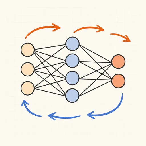
Backpropagation Step-by-Step
Walk through one forward and backward pass of a tiny neural network, number by number.

Handwritten Digit Recognizer
Draw a digit and watch a neural network trained on MNIST recognize it live in your browser.
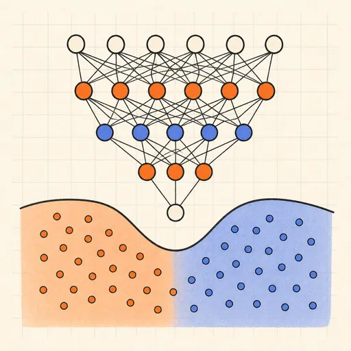
Neural Network Playground
Train a tiny neural network live in your browser and watch its decision boundary learn four classic datasets.
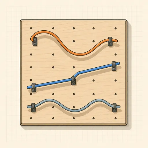
Activation Function Explorer
Compare sigmoid, tanh, ReLU and friends with their derivatives, and see why deep gradients vanish.
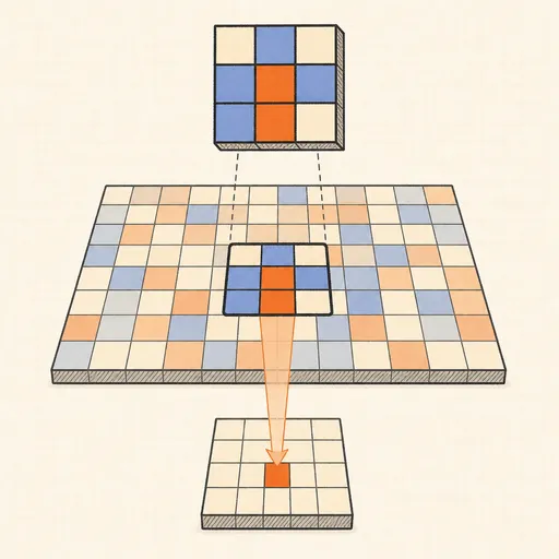
Convolution Filter Visualizer
Slide a 3×3 kernel over an image and watch convolution, ReLU and max-pooling build the output pixel by pixel.
Self-Attention Visualizer
See how Transformer tokens attend to each other with arcs, heatmaps, heads and causal masks.