Gradient Boosting, Step by Step
After reading this you will be able to build a gradient boosting regressor by hand: fit a mean, fit shallow trees to residuals, scale them by a learning rate, and read the train/test error curves to know when to stop.
What gradient boosting does
Gradient boosting builds one strong model by adding many weak ones. Each weak model is a shallow regression tree. On its own, a depth-2 tree can only split a line into at most four flat pieces, so it fits the data badly. Add fifty of them, each correcting the last one's mistakes, and the sum bends into a smooth curve.
Here is the hook. Suppose the true signal is a sine wave and you have 40 noisy points. Stage one predicts a single flat line at the average y value, say 0.02. That line is wrong almost everywhere. So you measure how wrong it is at each point (the residual), fit a small tree to those residuals, and add a fraction of it to the prediction. Repeat. The prediction stops being flat, grows a bump where the sine peaks, dips where the sine troughs, and after 60 stages traces the wave closely.
The word "gradient" is not decoration. For squared-error loss, the residual y - F(x) is exactly the negative gradient of the loss with respect to the prediction. Fitting the next tree to the residuals is fitting it to the direction that reduces loss fastest. That is why the method generalizes to other losses: you always fit the next tree to the negative gradient.
When to use it, and when not to
Gradient boosting is the default choice for tabular data with mixed feature types and moderate size, tens of thousands to a few million rows. It handles nonlinear relationships and interactions without you specifying them, and it usually beats a single tree or a linear model on accuracy.
It is a poor first choice in three cases. First, when you have very little data: a boosted ensemble of hundreds of trees will memorize 40 points long before it learns the pattern. Second, when you need a model you can read off in one glance; a single decision tree or a linear regression is far more transparent. Third, on raw images, audio or long text, where neural networks exploit structure that trees cannot see.
Boosting and bagging both average many trees, but they differ. A random forest grows deep trees independently on bootstrap samples and averages them to cut variance. Boosting grows shallow trees sequentially, each fixing the previous errors, to cut bias. Forests are hard to overfit by adding trees; boosting overfits readily, which is the pitfall this page keeps returning to.
The update rule and why it works
Start with a constant model. For squared loss the best constant is the mean of the targets:
Here n is the number of training points and \bar{y} their average. That is the flat line every squared-loss ensemble starts from.
At stage m, compute the residual at each point, fit a shallow tree h_m to those residuals, and add a shrunken copy:
\nu is the learning rate (shrinkage), a number in (0, 1]. The residual that h_m is fitted to is
For squared loss the per-point loss is \tfrac{1}{2}(y_i - F(x_i))^2, whose derivative with respect to the prediction F(x_i) is -(y_i - F(x_i)) = -r_{i,m}. The residual is the negative gradient, so each stage is one step of gradient descent in function space, with the tree acting as the step direction and \nu as the step size.
A small \nu, say 0.1, takes small steps. You need more stages to reach a given training fit, but each step is gentle and the final ensemble usually generalizes better. A large \nu, say 1.0, races to fit the training set and reaches the U-shaped bottom of test error sooner, then overshoots into noise.
Four stages on a tiny sine, by hand
Take six points from a sine, no noise, so you can check every number. The demo starts from these x values evenly spaced on [0, 1] with y = \sin(2\pi x), rounded to three digits.
| x | y | F_0 | r = y - F_0 |
|---|---|---|---|
| 0.0 | 0.000 | 0.000 | 0.000 |
| 0.2 | 0.951 | 0.000 | 0.951 |
| 0.4 | 0.588 | 0.000 | 0.588 |
| 0.6 | -0.588 | 0.000 | -0.588 |
| 0.8 | -0.951 | 0.000 | -0.951 |
| 1.0 | 0.000 | 0.000 | 0.000 |
- The mean of
yis0.000, so F_0(x) = 0 everywhere. Residuals equaly. Training MSE is the mean of y^2:(0 + 0.904 + 0.346 + 0.346 + 0.904 + 0)/6 = 0.4165. - Fit a decision stump (one split) to the residuals. The best split is at
x = 0.5. Points with x \lt 0.5 have residuals0, 0.951, 0.588, mean0.513. Points with x \ge 0.5 have residuals-0.588, -0.951, 0, mean-0.513. So h_1 outputs+0.513on the left,-0.513on the right. - Update with \nu = 0.5: F_1 = F_0 + 0.5 \cdot h_1. Left points get
+0.257, right points get-0.257. - New residuals at
x = 0.2:0.951 - 0.257 = 0.694. Atx = 0.8:-0.951 + 0.257 = -0.694. The two flat pieces already cut the training MSE from0.4165to0.2795, a 33% drop from one stump scaled by half.
Keep going and the next stumps split at 0.3 and 0.7, carving the line into finer steps that hug the sine. A depth-2 tree would make two splits per stage and get there in fewer stages, which is the trade the depth toggle in the tool demonstrates.
Watch the learning rate trade steps for smoothness
The single most instructive knob is \nu. Small values need more stages but land softer; large values fit fast and overfit fast. Move the slider and watch both the stage count needed and the shape of the test error curve.
Reading the train and test error curves
The tool draws two curves against stage number. The training MSE only ever decreases, because each stage takes a gradient step that reduces training loss. That curve alone tells you nothing about overfitting; it will happily reach zero if you add enough trees.
The test MSE is the one that matters. It falls at first, because early trees learn real structure that transfers to unseen points. It reaches a minimum, then rises, because later trees fit noise specific to the training set. The stage of the minimum is where you should stop. Real libraries call this early stopping: they watch a validation score and halt when it stops improving.
Report the test MSE at its minimum, not at the last stage. In the chart the minimum near stage 29 is 0.0401, while stage 71 has risen to 0.0802, double the error. Two ensembles built the same way can differ twofold in quality purely by where you stopped.
Common mistakes
Reading only the training curve. A training MSE marching toward zero looks like success and is often the opposite. Always hold out test points and watch their error.
Pushing the learning rate up to save stages. A rate of 1.0 reaches a low training error in a dozen stages, but its test minimum is both higher and narrower, so it is easy to overshoot. A rate of 0.1 with more stages is the safer default.
Using deep trees as the base learner. Boosting works because each tree is weak. Depth-2 trees make small corrections. A depth-8 tree can fit most of the residual noise in one stage, and the ensemble overfits almost immediately.
Confusing boosting with bagging. If you find yourself adding more trees to reduce variance and expecting the error to keep falling, you are thinking of a forest. In boosting, more trees eventually increase test error.
The step function target exposes a real limitation. Trees predict a constant within each leaf, so a boosted ensemble approximates the smooth sine with a staircase. On a true step function it fits the jump cleanly, but on a kinked or curved target you will always see small flat steps in the blue curve. That is the base learner showing through, not a bug.
Related tools on this site
Boosting stacks the base learner from the Decision Tree Builder, so build a single stump there first to see what one stage adds. Contrast it with the Random Forest Voting tool to feel the difference between averaging independent trees and stacking sequential ones. The overfitting story here is the same one told with polynomials in the Overfitting Sandbox. For the gradient-descent view of a simpler model, the Linear Regression Playground shows the loss surface directly, and the Logistic Regression Playground extends that idea to classification.
Frequently asked questions
Why does the ensemble always start as a flat line?
With squared loss the best constant prediction is the mean of the targets, and stage zero is exactly that constant. So the first prediction is a horizontal line at \bar{y}. Every later stage bends it away from flat.
What is the difference between the residual and the gradient?
For squared-error loss they are the same up to sign. The gradient of \tfrac{1}{2}(y - F)^2 with respect to F is -(y - F), so the residual y - F is the negative gradient. Fitting a tree to residuals is a gradient step. For other losses, such as absolute error, the negative gradient is not the plain residual, which is why the general method fits the gradient.
How many stages should I use?
Enough to reach the minimum of the test curve, no more. That number depends on the learning rate and noise. In the chart above, learning rate 0.3 reaches its minimum near stage 29; halving the rate to 0.15 would roughly double that.
Does depth-2 versus a stump change the final fit?
Both can fit the same curve, but a depth-2 tree makes two splits per stage and covers ground faster, so it needs fewer stages. A stump makes one split per stage and needs more. The depth toggle in the tool lets you watch a stump take two or three times as many stages to reach the same shape.
Can boosting overfit even with no noise?
With perfectly clean data and few points, the training error simply drops toward zero and the test error can stay low, because there is no noise to fit. Overfitting shows up once the data carries noise: later trees start modeling the noise, and test error turns upward. Raise the noise slider in the tool to see the U-shape deepen.
Related tools
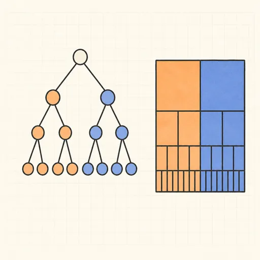
Decision Tree Builder
Grow a CART decision tree split by split and watch the partition map and tree diagram build together.
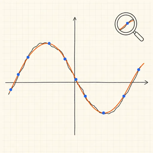
Function Sketch Finder
Sketch a curve on a zoomable coordinate grid and search dozens of function families for the equations that fit it best.
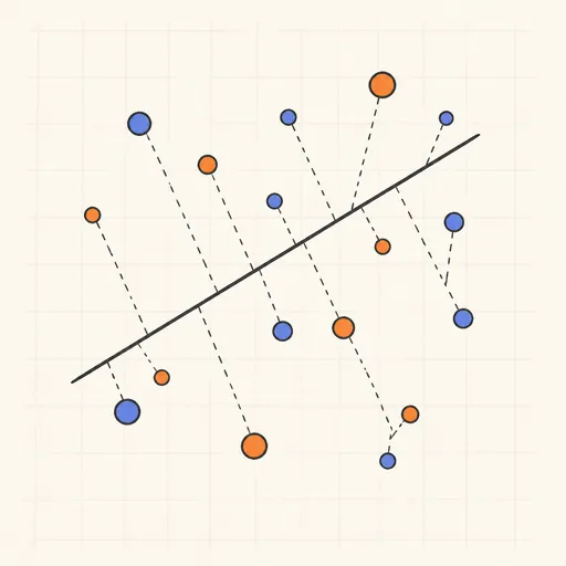
Linear Regression Playground
Place points, watch the least-squares line follow, and see gradient descent crawl across the loss surface.
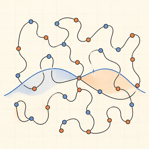
Overfitting Sandbox
Crank a polynomial’s degree on noisy data and watch the train/test error curves split apart.
Logistic Regression Playground
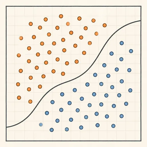
Paint two classes of points and watch logistic regression carve out its probability boundary by gradient descent.

Naive Bayes Classifier Demo
Score your own message with a word-count spam filter, or watch Gaussian naive Bayes classify 2D points.