Time Series Lab: Decomposition, ETS & ARIMA Forecast
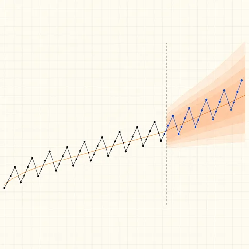
A complete forecasting workbench in the browser. Paste or drop a CSV with a date column (or plain values), and the lab detects the frequency and seasonal period, splits the series into trend, seasonal pattern and remainder with an STL-style loess decomposition, fits the best exponential-smoothing state-space model (ETS: level, damped trend, additive or multiplicative season) and the best seasonal ARIMA by AICc, and forecasts ahead with 80% and custom prediction intervals. Rolling-origin cross-validation then scores every model against naive, seasonal-naive and drift baselines (MAE, RMSE, MAPE, MASE), so the headline forecast is the one that actually predicted best out of sample — not the one that fit best in hindsight.
Read the full guide to this tool
Results
Notes
- Decomposition is STL-style: a periodic seasonal component and a loess trend, iterated with bisquare robustness weights so outliers land in the remainder. Strengths Fₜ and Fₛ are Wang–Smith–Hyndman measures: 1 − Var(remainder)/Var(component + remainder).
- ETS variants tried: no / additive / damped trend × no / seasonal component, all with additive errors, fitted by maximising the Gaussian likelihood over smoothing parameters and initial states; the lowest AICc wins.
- ARIMA: seasonal differencing when seasonal strength exceeds 0.64, ordinary differencing until a KPSS test accepts stationarity, then (p,q)≤(3,3) and seasonal (P,Q)≤(1,1) screened by Hannan–Rissanen regressions and the best six refitted by conditional least squares. AICc is only comparable between models with the same differencing.
- MASE scales errors by the in-sample seasonal-naive error: below 1 beats copying last season; above 1 you would have done better with no model.
- A Ljung–Box p-value under 0.05 says the residuals still carry structure the model missed — the intervals are then too narrow.
Explore the idea
Related tools

Descriptive Statistics Calculator
Mean, median, quartiles, variance, skewness, outliers and more.
Kaplan–Meier Survival Calculator
Survival curve, life table and median survival from time-to-event data with censoring.

Outlier Detector
Grubbs' test, Tukey fences and z-scores on your data.

Autocorrelation Calculator
ACF by lag with white-noise bands and the Ljung–Box test.

Covariance Calculator
Sample and population covariance with Pearson correlation.

Percentile Calculator
Find the value at a percentile, or the rank of a value.