Vanishing and Exploding Gradients, Explained
After reading this you will be able to predict, from the activation and the weight initialization alone, whether the early layers of a deep network get a usable training signal, and you will be able to check the prediction with a few multiplications by hand.
What the problem is
Backpropagation trains a network by sending an error signal from the output layer back toward the input. That signal reaches an early layer only after passing through every layer above it. Each pass multiplies the signal by a factor. Multiply enough numbers below 1 together and the result shrinks toward zero. Multiply enough numbers above 1 and it grows without bound.
Here is the hook. A sigmoid activation has a derivative that never exceeds 0.25. Stack 20 sigmoid layers with poorly scaled weights and the gradient reaching layer 1 can be smaller than the gradient at layer 20 by a factor near 0.25^{20} \approx 9 \times 10^{-13}. The early layers barely move. The loss curve flattens while the network is still wrong. That is a vanishing gradient.
The tool trains a genuinely deep multilayer perceptron (2 to 30 hidden layers, 16 units wide) on a two-blob classification task and draws one horizontal bar per layer for the mean absolute gradient on a log scale. You watch the early bars starve or blow up as SGD runs.
When this matters and when it does not
The product-of-factors problem is a property of depth. A network with 2 or 3 hidden layers rarely suffers from it, because a short product of moderate factors stays in a reasonable range. The trouble grows with the number of layers, so it dominates the design of very deep convolutional networks, recurrent networks unrolled over long sequences, and any architecture with dozens of stacked transformations.
You do not need to worry about it when your model is shallow, when your activations keep derivatives near 1 across their useful range, and when your initialization is scaled to the layer width. Modern defaults (He initialization with ReLU, plus batch normalization or residual connections) were built precisely to keep the product near 1, so with those defaults the raw problem is mostly tamed. This tool exists to show you what those defaults are protecting you from.
The formula and the intuition behind it
Consider a chain of layers where layer \ell computes a_\ell = f(z_\ell) with z_\ell = w_\ell a_{\ell-1}. The gradient of the loss with respect to an early activation is a product running down through every layer above it:
Here L is the number of layers, w_\ell is the weight (or, in the full network, a weight matrix), and f'(z_\ell) is the activation derivative at that layer. The single factor that decides the fate of the whole product is the typical size of w_\ell \cdot f'(z_\ell). Call it r. If r \lt 1 the product decays like r^{L}. If r \gt 1 it grows like r^{L}. Only r \approx 1 keeps every layer trainable.
Two levers set r: the activation caps f', and the initialization sets the scale of w. Sigmoid caps f' at 0.25, tanh at 1, ReLU at 1 (but only for half its inputs). Xavier draws weights with variance 1/n; He uses 2/n to make up for ReLU zeroing half the signal.
A worked example you can reproduce
Use the demo defaults and treat each layer as one representative factor. Compare sigmoid with naive N(0,1) init against ReLU with He init, both at depth 20 and width 16.
Sigmoid, naive init, 20 layers
- Sigmoid derivative peaks at
0.25. Once activations saturate, a realistic average is closer to0.15, but take the generous peak. - Naive N(0,1) weights summed over 16 inputs push z into the flat tails, so the effective per-layer factor r = w \cdot f' sits below
1. Take r = 0.7 as an optimistic estimate. - Over 20 layers the product is 0.7^{20} \approx 8 \times 10^{-4}.
- The gradient at layer 1 is therefore about 1200 times smaller than at layer 20. On the log-scale bar chart that is roughly 3 decades of difference, and it grows worse once saturation drives r below
0.7.
ReLU, He init, 20 layers
- He init sets weight variance to 2/n = 2/16 = 0.125, so a typical weight magnitude is \sqrt{0.125} \approx 0.354.
- ReLU passes its input unchanged where active (f' = 1) and blocks it otherwise (f' = 0), active for about half its inputs.
- The variance-preserving design makes the expected per-layer factor r \approx 1. The product 1^{20} = 1 stays flat.
- On the bar chart every layer shows a bar of similar length, and the loss actually falls.
Reading the bars and the ratio
The tool plots the mean absolute gradient per layer on a log scale, so equal bar lengths mean equal orders of magnitude. Healthy training looks like bars of comparable length across all layers. Vanishing looks like a staircase that shrinks steeply toward the input. Exploding looks like the mirror image, with the early bars running off the scale before the loss turns to NaN.
The single number to watch is the first-to-last-layer gradient ratio. Divide the mean absolute gradient at layer 1 by the mean absolute gradient at layer L. A ratio near 1 (say between 0.1 and 10) means every layer learns at a similar pace. A ratio of 10^{-3} means the first layer receives a thousandth of the last layer's signal and is effectively frozen. A ratio above 10^{3} is the warning sign for an explosion.
Common mistakes
The first mistake is blaming the learning rate. When the early-layer gradients are a thousand times too small, raising the learning rate does not fix the ratio, it just makes the late layers oscillate while the early ones stay stuck. Fix the product first, then tune the step size.
The second is trusting a flat loss curve. A vanishing-gradient run and a converged run both show a flat loss, but for opposite reasons. Check the per-layer bars and the ratio, not the loss alone.
Do not read the browser demo as a benchmark. It trains a 16-unit-wide MLP on two Gaussian blobs. The mechanism it shows (a product of factors deciding gradient scale) is exactly the same one that governs a 100-layer production network, but the numbers, the training time, and the exact thresholds do not transfer. Treat it as a microscope on the mechanism, not a measurement of any real model.
The third is switching to He init while keeping tanh, or Xavier while keeping ReLU. Xavier's 1/n variance is derived for activations symmetric around zero with derivative near 1, which fits tanh. He's 2/n compensates for ReLU discarding half its inputs. Mismatch the pair and you drift off r = 1.
Related tools
To see the mechanics of the backward pass that produces these gradients, work through the Backpropagation Step-by-Step tool one number at a time. To study why each activation caps its derivative where it does, compare curves in the Activation Function Explorer. For a shallow network where gradient scaling is not yet a problem, train the Neural Network Playground and watch its decision boundary. Recurrent networks unroll into very deep chains, so the same product problem drives the Character RNN Text Generator, and gating was one of the answers to it.
Frequently asked questions
Why does sigmoid vanish faster than tanh?
The sigmoid derivative peaks at 0.25 while the tanh derivative peaks at 1. Even with ideal weights, a sigmoid chain multiplies by at most 0.25 per layer, so 0.25^{10} \approx 10^{-6} vanishes far sooner than a tanh chain kept near 1.
What actually stops exploding gradients in practice?
Gradient clipping caps the update norm at a threshold, so a factor above 1 can no longer multiply the step to infinity. Combined with scaled initialization it keeps a run from producing NaN. Clipping treats the symptom; correct init treats the cause.
Does batch normalization fix vanishing gradients?
It helps by rescaling each layer's activations to keep the per-layer factor near 1, which shortens the effective distance the product can drift from 1. It is not a full replacement for good initialization, but it makes deep training far more forgiving.
Is a ratio of exactly 1 the goal?
No. Any ratio within about one order of magnitude, say 0.1 to 10, means every layer trains at a usable pace. The danger begins when the ratio reaches 10^{-3} or 10^{3}, where the extreme layers are either frozen or diverging.
Related tools
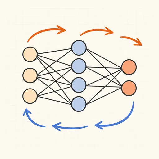
Backpropagation Step-by-Step
Walk through one forward and backward pass of a tiny neural network, number by number.

Handwritten Digit Recognizer
Draw a digit and watch a neural network trained on MNIST recognize it live in your browser.
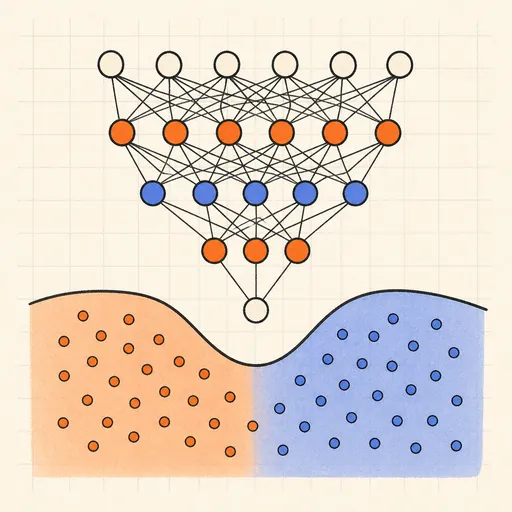
Neural Network Playground
Train a tiny neural network live in your browser and watch its decision boundary learn four classic datasets.
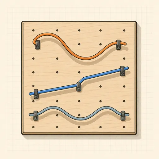
Activation Function Explorer
Compare sigmoid, tanh, ReLU and friends with their derivatives, and see why deep gradients vanish.
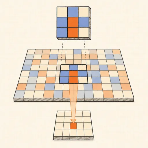
Convolution Filter Visualizer
Slide a 3×3 kernel over an image and watch convolution, ReLU and max-pooling build the output pixel by pixel.
Hopfield Network
Store pixel patterns in a Hopfield memory, corrupt them, and watch the network recall the original.