Regularization: L1, L2 and Dropout
After reading this you will know exactly what the L2 penalty, the L1 penalty and dropout do to a network's weights, how to read the train/test gap that signals overfitting, and how to pick a regularization strength that closes that gap without crippling the model.
What regularization is
A neural network with more free parameters than the data needs will fit the noise, not just the signal. The 2-8-8-2 network in this demo has 2 inputs, two hidden layers of 8 units each, and 2 outputs. Count its weights: 2×8 + 8×8 + 8×2 = 16 + 64 + 16 = 96, plus 18 biases, so 114 numbers in total. If you train it on only 100 noisy points, there is plenty of capacity to trace a wiggly boundary that curls around every stray point.
Regularization is the set of methods that discourage that wiggling. It does not remove capacity. It changes the loss so that a simpler model is preferred unless the data strongly demands complexity. Three methods appear here. L2 shrinks every weight a little toward zero. L1 drives many weights exactly to zero. Dropout randomly silences hidden units during training so no single unit can dominate.
The hook: train the two-moons dataset with noise 0.35 and no regularization, and you will typically see training accuracy reach 0.99 while test accuracy stalls near 0.83. Turn L2 up to \lambda = 0.01 and both settle around 0.90. The network got worse at the training points and better at the ones it had never seen.
When to use it, and when not
Reach for regularization when the gap between training and test accuracy is large and growing. If training accuracy is 0.99 and test accuracy is 0.82, that 17-point gap is the symptom. If both sit at 0.72, the model is underfitting and adding a penalty will only make it worse. Regularization trades a small amount of training fit for a large amount of test fit, and there is no gain to trade when there is no overfitting to fix.
Change one knob at a time. If you raise L2, raise L1 and add dropout all at once, you cannot tell which one helped. Start from zero regularization, confirm the network overfits, then increase a single penalty until the test curve stops improving.
Choose by the shape you want in the weights. L2 keeps every weight but makes them small and smooth, which suits problems where all inputs matter a little. L1 zeroes out weights it can spare, which suits problems where you suspect many inputs are useless and you want a sparse, readable model. Dropout is cheap insurance against any one unit becoming a single point of failure, and it stacks with either penalty.
The formulas and the intuition
Start from the plain training loss L_0, the cross-entropy over the training points. Each method modifies either the loss or the forward pass.
L2, also called weight decay
Here w_i is each individual weight and \lambda is the strength. The gradient of the penalty with respect to w_i is 2\lambda w_i, so a gradient step subtracts a piece proportional to the weight itself. Folding the constant into \lambda, the update is:
The factor (1 - \eta\lambda) multiplies the weight every step, so a weight of 2.0 under learning rate \eta = 0.1 and \lambda = 0.01 shrinks to 2.0 × (1 − 0.001) = 1.998 from the penalty alone. The pull is proportional to size, so large weights shrink fast and tiny weights barely move. That is why L2 rarely sends a weight all the way to zero.
L1
The derivative of |w| is \text{sign}(w), which is +1 or -1 regardless of size. So the penalty step is a constant nudge toward zero:
A weight of 0.005 under \eta = 0.1 and \lambda = 0.01 loses 0.1 × 0.01 × 1 = 0.001 per step from the penalty. Unless the data pushes back hard enough to overcome that fixed 0.001, the weight crosses zero and stays clamped there. That constant pull is exactly why L1 produces sparse networks while L2 does not.
Dropout
Dropout changes the forward pass, not the loss. With rate p, each hidden unit is set to zero independently with probability p on each training step. To keep the expected sum of activations unchanged, the surviving units are scaled up by 1/(1-p):
Here a_j is the unit's activation, m_j is 0 or 1, and the 1/(1-p) factor is the inverted scaling. With p = 0.5 a surviving unit is doubled, so if 4 of 8 units survive, their scaled sum matches the expected sum of all 8. At test time you drop nothing and scale nothing: the network runs at full width and behaves like an average over the many thinned networks seen during training.
A worked example on the demo data
Press the demo button to load the field defaults: the two-moons dataset, noise 0.35, an 80/20 train/test split, and the 2-8-8-2 network. The numbers below trace what you should see as you sweep the L2 strength.
Sweeping L2 on two moons
- Set all three regularizers to zero and train to convergence. Training accuracy climbs to about
0.99. Test accuracy peaks near0.85then drifts down to0.83as the boundary curls around noise points. The gap is0.16. - Set \lambda = 0.001. Weights shrink slightly. The gap narrows to about
0.11, with training at0.96and test at0.85. - Set \lambda = 0.01. Training drops to
0.92, test rises to0.90. The gap is0.02. This is close to the sweet spot. - Set \lambda = 0.1. Now the penalty dominates. Weights are so small the boundary flattens toward a straight line. Training and test both fall to about
0.80. You have moved from overfitting to underfitting.
The lesson is the U shape: too little regularization overfits, too much underfits, and the best test accuracy sits at an intermediate strength you find by sweeping.
Reading the train and test curves
The most useful plot in the demo is the pair of accuracy curves over training steps. Read them together, never alone.
| Training acc | Test acc | Gap | Diagnosis | Action |
|---|---|---|---|---|
| 0.99 | 0.83 | 0.16 | Overfitting | Add regularization |
| 0.92 | 0.90 | 0.02 | Well fit | Leave it |
| 0.80 | 0.80 | 0.00 | Underfitting | Reduce penalty or add capacity |
| 0.98 | 0.97 | 0.01 | Easy problem | Nothing needed |
Also watch the weight histogram. Under L2 the histogram contracts toward zero but stays a smooth bell, and few or no weights land exactly at zero. Under L1 a tall spike grows at zero: with \lambda = 0.01 you can drive 40 percent or more of the 96 weights to exactly zero, and the demo reports that near-zero percentage live. A network with half its weights zeroed is doing the same job with half the parameters.
Dropout makes the training accuracy curve noisy and often lower than the test curve, because at train time the network runs thinned while at test time it runs full. A training accuracy below test accuracy is normal with dropout and is not a bug.
Common mistakes
The errors below account for most confusion people report with these three methods.
- Regularizing the biases
- Penalties should apply to weights, not biases. A bias shifts the whole decision boundary and shrinking it toward zero just moves the boundary off-center for no benefit. This demo penalizes weights only.
- Setting lambda by training loss
- Adding a penalty raises the total loss by design, so a higher lambda always looks worse on training loss. Judge lambda by test accuracy, never by the loss value.
- Comparing L1 sparsity at different lambdas
- The near-zero percentage only means something at a fixed strength. At \lambda = 0.001 you might see 5 percent of weights at zero; at \lambda = 0.02, 60 percent. Sparsity is a function of the pull, not a property of the data alone.
- Using dropout at test time
- Dropout runs during training only. If you keep dropping units at test time your predictions become random and accuracy swings. With inverted scaling the test network is used as-is.
- Cranking every knob together
- Strong L1 plus strong L2 plus p = 0.7 dropout can push a network to near-constant output. If test accuracy collapses toward 0.50 on a two-class problem, you have over-regularized.
Related tools
Regularization sits inside the training loop, so the neighboring demos help you see the parts it touches. Build the base network and its boundary in the Neural Network Playground, then follow a single weight update by hand in Backpropagation Step-by-Step to see where the (1 - \eta\lambda) factor enters. The choice of activation interacts with regularization through the gradient scale, which you can explore in the Activation Function Explorer and, for deeper networks, in Vanishing & Exploding Gradients. To see regularization at real scale on images, train the Handwritten Digit Recognizer.
Frequently asked questions
What is the difference between L1 and L2 in one sentence?
L2 pulls each weight toward zero by an amount proportional to its size, so all weights shrink but stay nonzero, while L1 pulls by a constant amount, so small weights reach exactly zero and the network becomes sparse.
How do I choose the regularization strength?
Sweep it. Start at zero, confirm the train/test gap is large, then increase lambda in factors of about 3 (0.001, 0.003, 0.01, 0.03) and keep the value that gives the highest test accuracy. In this demo that peak is near \lambda = 0.01 for two moons at noise 0.35.
Can I use L1, L2 and dropout at the same time?
Yes, they are independent and combine cleanly. In practice a small L2 plus modest dropout (p = 0.2 to 0.5) is a common pairing. Add them one at a time so you can attribute each change in the test curve.
Why does dropout make training accuracy look worse than test accuracy?
During training the network runs with units randomly silenced, so it is a weaker, thinner model. At test time all units are active and scaled correctly, so the full network scores higher. The reversed gap is expected.
Does regularization help if my model is underfitting?
No. If training and test accuracy are both low and close together, the model lacks capacity or has not trained long enough. Adding a penalty removes capacity and makes both numbers worse. Reduce the penalty or add units instead.
What does the near-zero percentage in the demo mean?
It is the fraction of the 96 weights whose magnitude is below a small threshold, essentially zero. Under L2 it stays near a few percent. Under L1 with a moderate lambda it can exceed 40 percent, which is the visible signature of the sparsity L1 induces.
Related tools
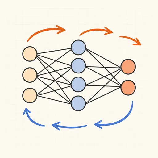
Backpropagation Step-by-Step
Walk through one forward and backward pass of a tiny neural network, number by number.

Handwritten Digit Recognizer
Draw a digit and watch a neural network trained on MNIST recognize it live in your browser.
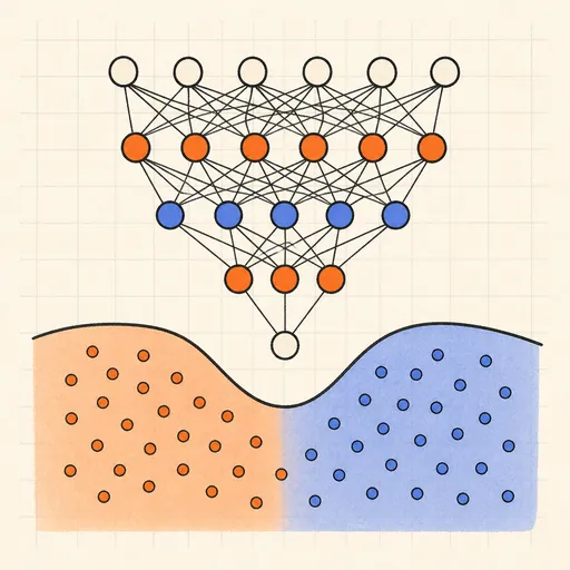
Neural Network Playground
Train a tiny neural network live in your browser and watch its decision boundary learn four classic datasets.
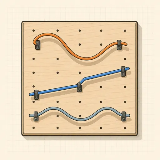
Activation Function Explorer
Compare sigmoid, tanh, ReLU and friends with their derivatives, and see why deep gradients vanish.
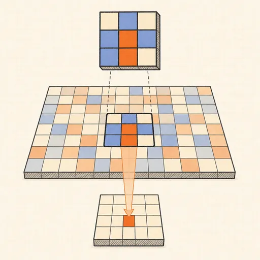
Convolution Filter Visualizer
Slide a 3×3 kernel over an image and watch convolution, ReLU and max-pooling build the output pixel by pixel.

Hopfield Network
Store pixel patterns in a Hopfield memory, corrupt them, and watch the network recall the original.