Sorting Algorithms, Watched Step by Step
After reading this you can predict how many comparisons and swaps each classic sorting algorithm needs on a given array, and explain why an O(n log n) sort pulls ahead of an O(n²) sort as the array grows.
What a sorting algorithm actually does
Sorting means rearranging a list so its elements sit in order, usually smallest to largest. Every algorithm in this visualizer reaches the same final arrangement. What differs is the path: how many pairs of elements it compares, and how many times it moves elements around.
Watch bubble sort on a shuffled bar chart and the pattern is obvious. It walks left to right, comparing each bar with its neighbour, and swaps them if they are out of order. The largest bar "bubbles" to the far right on the first pass. The second pass fixes the second largest, and so on. It is easy to read but slow: on 50 bars it can run several thousand comparisons.
Now watch merge sort on the same 50 bars. It splits the array in half, sorts each half, then merges the two sorted halves. The merge does the real work, weaving two ordered lists into one. On those same 50 bars it needs roughly 280 comparisons. Same input, same output, an order of magnitude less work.
The seven algorithms at a glance
The tool animates seven sorts. Three are quadratic and simple. Four are faster and more structured. Keep the two groups separate in your head.
| Algorithm | Best | Average | Worst | Extra memory | Stable |
|---|---|---|---|---|---|
| Bubble | n | n² | n² | 1 | yes |
| Selection | n² | n² | n² | 1 | no |
| Insertion | n | n² | n² | 1 | yes |
| Shell | n log n | ~n^1.3 | n² | 1 | no |
| Merge | n log n | n log n | n log n | n | yes |
| Quick | n log n | n log n | n² | log n | no |
| Heap | n log n | n log n | n log n | 1 | no |
Stable means equal elements keep their original relative order. That matters when you sort records by one field and want ties to stay in their earlier order. Extra memory counts space beyond the input array: merge sort needs a full copy, heap sort needs almost nothing.
When to reach for each one
Use insertion sort for small arrays (say fewer than 20 elements) or for data that is already nearly sorted. It is nearly linear on almost-ordered input. Many real libraries switch to insertion sort for small subarrays inside a bigger merge or quick sort, because its low overhead beats the recursion cost.
Use merge sort when you need stability guaranteed, or when worst-case timing must stay predictable. It never degrades to n². The price is the extra array of size n.
Use quicksort as the general default for in-memory sorting. Its average behaviour is excellent and its constant factors are small. But naive quicksort, which always picks the first or last element as pivot, degrades to n² on already-sorted input. Real implementations pick the pivot with care.
Do not judge an algorithm from one starting arrangement. Naive quicksort looks brilliant on shuffled data and terrible on sorted data. Insertion sort looks slow on reversed data and superb on nearly sorted data. Run each sort on all four arrangements in the tool before drawing conclusions.
Why n log n beats n squared
The quadratic sorts do a fixed fraction of n^2 comparisons. Bubble and selection sort, for example, compare roughly every pair once:
Here n is the number of elements and C is the comparison count. For n = 50 that gives \frac{50 \cdot 49}{2} = 1225 comparisons.
The divide-and-conquer sorts split the problem in half about \log_2 n times, and each level does about n work:
For n = 50, \log_2 50 \approx 5.64, so 50 \cdot 5.64 \approx 282 comparisons. That is the 1225 versus 282 gap you see in the tool. The gap widens fast. At n = 1000 the quadratic count is 499500 while n \log_2 n \approx 9966, a factor of about 50.
A worked example on the demo data
Insertion sort on eight shuffled bars
Take a small shuffled array of eight heights: [5, 2, 8, 1, 9, 3, 7, 4]. Insertion sort keeps a sorted region on the left and pulls the next element back into place.
- Start with
5alone as sorted. Sorted region:[5]. - Insert
2. Compare with 5, 2 is smaller, shift 5 right. 1 comparison, 1 swap. Now[2, 5]. - Insert
8. Compare with 5, 8 is larger, stop. 1 comparison, 0 swaps. Now[2, 5, 8]. - Insert
1. Compare with 8, 5, 2, all larger, shift all three. 3 comparisons, 3 swaps. Now[1, 2, 5, 8]. - Insert
9. Compare with 8, larger, stop. 1 comparison, 0 swaps. Now[1, 2, 5, 8, 9]. - Insert
3. Compare with 9, 8, 5, then 2 stops it. 4 comparisons, 3 swaps. Now[1, 2, 3, 5, 8, 9]. - Insert
7. Compare with 9, 8, then 5 stops it. 3 comparisons, 2 swaps. Now[1, 2, 3, 5, 7, 8, 9]. - Insert
4. Compare with 9, 8, 7, 5, then 3 stops it. 5 comparisons, 4 swaps. Final:[1, 2, 3, 4, 5, 7, 8, 9].
Total: 1+1+3+1+4+3+5 = 18 comparisons and 1+0+3+0+3+2+4 = 13 swaps. The theoretical worst case for eight elements is \frac{8 \cdot 7}{2} = 28 comparisons, which you would hit on a fully reversed array. This shuffled input needed only 18, because insertion sort stops early whenever an element is already close to its place.
Reading the live counters
The tool tracks comparisons and swaps separately, and the split tells you something. Selection sort and bubble sort do about the same number of comparisons, but selection sort does far fewer swaps: it finds the minimum by comparing, then makes exactly one swap per pass, at most n-1 swaps total. Bubble sort can swap thousands of times on the same data.
That matters in the real world. If a comparison is cheap but moving an element is expensive (large records, slow storage), selection sort's low swap count can win despite equal comparison counts. Watch both counters, not just one.
Set the same array size and starting arrangement, then run two algorithms in turn and write down both counters. A table of your own numbers teaches more than any single animation. Try bubble versus selection on 50 reversed bars: similar comparisons, wildly different swap counts.
Common mistakes when reading the visualizer
The first mistake is trusting the animation speed as a measure of efficiency. Speed is just how fast the tool draws frames. The counters are the real measure. A sort that looks frantic may be doing fewer operations than a calm-looking one.
The second mistake is comparing algorithms on different data. If you shuffle between runs, the arrays differ and the counts are not comparable. Fix the array size and arrangement, and only then compare.
The third mistake is generalising from tiny arrays. At n = 10 the quadratic sorts do 45 comparisons and merge sort does 33, barely different. The whole point of asymptotic analysis appears only as n grows. Push the size up and the gap becomes stark.
The fourth mistake is forgetting that these are model counts. The tool counts comparisons and swaps, not wall-clock time, cache misses or branch mispredictions. Real performance on real hardware depends on all of those. The counters teach the shape of the growth, not the exact runtime of a compiled program.
Related tools
If sorting hooks you, several neighbouring tools build on the same ideas. The Big-O Complexity Race shows the growth curves behind this article directly, racing log n against n² and worse. The Pathfinding Visualizer and the Graph Algorithm Playground apply the same animate-the-algorithm approach to graphs. For divide-and-conquer of a different flavour, the Dynamic Programming Visualizer fills its tables cell by cell, and the Huffman Coding Visualizer builds an optimal tree from letter frequencies.
Frequently asked questions
Which sorting algorithm is fastest?
There is no single winner. On average, quicksort is the fastest general-purpose in-memory sort because its constant factors are small. But merge sort guarantees O(n log n) even in the worst case, and insertion sort beats everything on tiny or nearly sorted arrays. Match the algorithm to the data.
Why does quicksort sometimes do more comparisons than merge sort?
Both are O(n log n) on average, but the constants differ, and quicksort's count depends on pivot choice and input order. On a bad pivot sequence quicksort's count rises toward n². Merge sort's count barely moves regardless of input, which is why it looks steadier in the bar chart.
What does "stable" mean and why should I care?
A stable sort keeps equal elements in their original order. If you sort a list of people by age and two people are both 30, a stable sort leaves them in their earlier order. Merge, bubble and insertion sort are stable; selection, quick and heap sort are not.
Why is insertion sort nearly linear on sorted data?
Each element only needs comparing with the one to its left. If it is already larger, insertion sort stops immediately. On fully sorted input that is exactly n-1 comparisons and zero swaps, which is linear. Reverse the same array and every insertion shifts the whole sorted region, pushing the count to \frac{n(n-1)}{2}.
Do the comparison counts translate to real running time?
Roughly, but not exactly. Comparison and swap counts predict how the running time grows with n. They do not capture memory access patterns, cache behaviour or the cost of a single comparison, all of which affect a real program's speed. Treat the counters as a faithful guide to growth, not a stopwatch.
Related tools
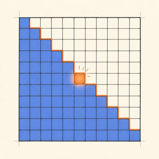
Dynamic Programming Visualizer
Watch edit distance and knapsack fill their tables cell by cell — dynamic programming with the lid off.
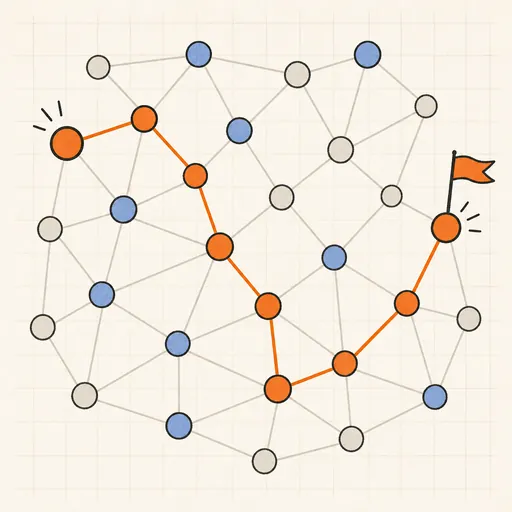
Graph Algorithm Playground
Build a graph by clicking, then watch BFS, DFS, Dijkstra and Prim explore it live.
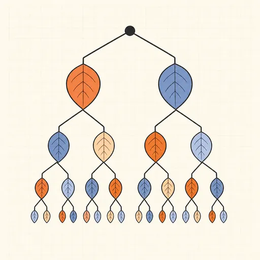
Huffman Coding Visualizer
Type any text and watch the optimal prefix code assemble itself as a tree, rare letters sinking deepest.
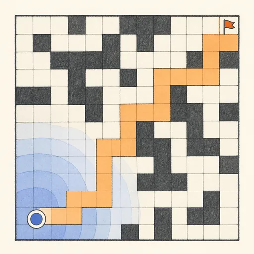
Pathfinding Visualizer
Draw walls and watch A*, Dijkstra, greedy and breadth-first search hunt for the shortest path.
Turing Machine Simulator
Watch a Turing machine read, write and shuffle along its tape — computation stripped to its atoms.
Hamming Code Playground
Flip any bit of a Hamming-encoded message and watch the parity checks point straight at the culprit.