How a GAN Trains, and Why It Collapses

After reading this you will understand the two-player game a GAN plays, be able to write down and check its loss functions by hand, and recognize mode collapse the moment it shows up in the 2D trainer.

What a GAN actually is

A generative adversarial network pairs two neural networks and makes them compete. The generator G takes random noise and outputs fake data points. The discriminator D looks at a point and outputs a number between 0 and 1: its estimate that the point came from the real dataset rather than from G.

The two are trained in opposite directions. D tries to score real points near 1 and fake points near 0. G tries to make its fakes score near 1, that is, to fool D. Neither has a fixed target. Each one's job depends on how good the other currently is.

In the 2D trainer the real data is a set of blue points arranged as a ring of 8 Gaussians, a spiral, or two moons. The generator maps 2D Gaussian noise through two hidden layers of 16 units to orange points. Run it on the ring and you will often see the orange cloud pile onto two or three of the eight blue blobs, ignore the rest, then hop to different blobs a few seconds later. That hopping is mode collapse, and it is the single most instructive failure a GAN shows.

When to reach for a GAN, and when not to

GANs learn to sample from a distribution. They do not give you a density value for a point, and they do not maximize a clean likelihood. If your goal is to draw new examples that look like your data, a GAN fits. If your goal is to score how likely a given point is, a GAN is the wrong tool.

The adversarial setup is worth the trouble when the data lives on a complicated, thin region of a high-dimensional space and you cannot write down its density. The cost is training instability. Because both networks move at once, the loss does not fall toward zero the way it does in ordinary supervised training. It oscillates, and you have to read other signals to know whether things are going well.

The loss functions, symbol by symbol

Write x for a real data point and z for a noise vector. The discriminator is trained to maximize its ability to tell the two apart:

Here D(x) is the discriminator's score for a real point, and D(G(z)) is its score for a fake point. The first term pushes D(x) toward 1 (so \log D(x) toward 0). The second term pushes D(G(z)) toward 0. The \mathbb{E} symbols are averages over a batch.

The generator's original objective was to minimize that same second term, which is the minimax form \log(1 - D(G(z))). In practice that gradient vanishes exactly when the generator is losing, which is when it needs a signal most. The 2D trainer uses the non-saturating loss instead:

This asks G to make D(G(z)) large. Check the gradient behavior with numbers. Suppose D is winning and scores a fake at D(G(z)) = 0.1. The minimax loss \log(1 - 0.1) = \log(0.9) = -0.105 is nearly flat there, so its slope is tiny. The non-saturating loss -\log(0.1) = 2.303 is large and steep. The generator keeps learning.

A worked step you can check

Work one discriminator update by hand on a two-point batch, using the ring setup that the demo button loads. Take one real point that D currently scores at D(x) = 0.6 and one fake point scored at D(G(z)) = 0.4.

The equilibrium, and why the curves oscillate

The game has a well-known balance point. When G reproduces the real distribution exactly, no discriminator can do better than guessing, so the best possible D outputs 0.5 everywhere. At that point both accuracies sit near 50%, and both loss curves hover rather than fall.

Plug D = 0.5 into the losses. The discriminator objective per point is (\log 0.5 + \log 0.5)/2 = -0.6931. The generator loss is -\log 0.5 = 0.6931. Watch for both curves settling into a band around those values. That is the sign of a healthy GAN, not a curve diving to zero.

How to read the trainer while it runs

Watch four things at once. The orange points show where G currently sends a fixed bank of noise. The faint heatmap behind them shows D's decision surface: dark where D says fake, light where it says real. The two loss curves show the tug of war. The status line reports how cleanly D separates real from fake.

On the ring of 8, healthy progress looks like orange points spreading toward several blue blobs while the heatmap stays roughly flat and gray. Mode collapse looks like orange points clustered on one or two blobs while the heatmap carves sharp dark valleys around the abandoned blobs. When you see the orange cluster jump from one blob to another, you are watching G chase whichever mode D just started punishing.

Common mistakes

The mistakes below all come from the same root: the balance between the two players.

Overtraining the discriminator

Set k high or the discriminator learning rate large and D becomes near perfect. It scores fakes at, say, 0.02. The generator gradient scales with D(G(z))(1 - D(G(z))) = 0.02 \times 0.98 = 0.0196, almost zero. The generator stalls.

Undertraining the discriminator

If D is barely trained it scores everything near 0.5 for the wrong reason. Its gradient points nowhere useful, so G chases a meaningless target and wanders.

Expecting the loss to converge

Treating a rising generator loss as failure. In a balanced GAN, G's loss going up often means D just improved, which is normal. Judge sample quality and mode coverage, not the loss alone.

Reading mode collapse as slow learning

A tight, confident orange cluster is not progress if it covers one blob out of eight. Coverage matters more than the sharpness of any single cluster.

Related tools on this site

A GAN is one way to learn to sample from a distribution. For a different mechanism that avoids the adversarial game entirely, try the Diffusion Model Toy, which learns to reverse a noising process step by step and tends to cover modes more evenly. For a non-neural generative model where you can see every transition probability by hand, see the Markov Chain Text Generator.

Related tools

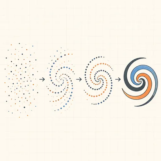
Diffusion Model Toy

Train a tiny denoising diffusion model and watch it turn pure noise back into a 2D shape.

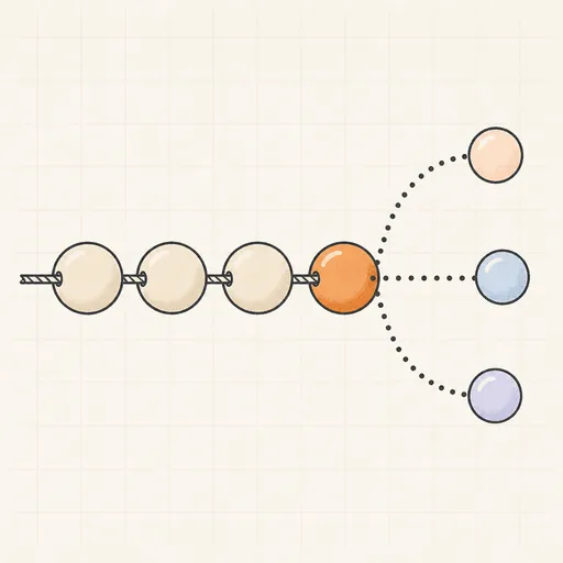
Markov Chain Text Generator

Train an order-k Markov chain on any text and generate new text one token at a time.

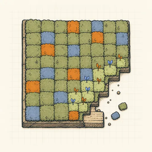
Neural Cellular Automata Sandbox

Grow, damage and heal living textures driven by a tiny convolutional network in every cell.

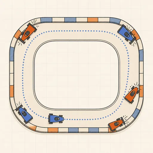
AI Learns to Drive (Neuroevolution)

Watch a population of neural-network cars evolve from crashing into corners to lapping a race track.

Backpropagation Step-by-Step

Walk through one forward and backward pass of a tiny neural network, number by number.

Decision Tree Builder

Grow a CART decision tree split by split and watch the partition map and tree diagram build together.