Denoising Diffusion Models, Explained
After reading this you can explain how a diffusion model turns Gaussian noise into a target shape, derive the noise-prediction loss it trains on, and reproduce the forward-process numbers from the toy by hand.
What a diffusion model does
A denoising diffusion model learns to generate data by reversing a slow corruption process. You start with a real point cloud, for example 500 points arranged in a spiral. You add a little Gaussian noise, then a little more, then more again, over 50 steps, until the cloud is indistinguishable from pure noise. That is the forward process, and it needs no learning: it is just adding noise on a fixed schedule.
The interesting direction is backward. If you could undo one step of noising, you could start from static and walk back to the shape. The model learns exactly that undo step. Concretely, given a noisy point and a timestep, it predicts the noise that was added. Subtract the predicted noise (scaled correctly), add a small amount of fresh noise, repeat 50 times, and a cloud of orange points condenses out of nothing into a spiral.
The hook to watch in the toy: the forward slider dissolves the blue cloud in real time, and the sampled orange cloud reassembles the same shape. The model never sees the shape as a whole. It only ever learns "given this messy point at step t, which noise vector do I remove?"
When this approach fits, and when it does not
Diffusion suits problems where you want to sample new data that resembles a training distribution and where the data is continuous. Images, audio and 2D point clouds fit well. The training objective is a plain regression loss, so it is stable: there is no adversarial game to balance. Compare that with the GAN Trainer (2D), where a generator and discriminator fight and can collapse onto a single mode.
Diffusion is a poor fit when you need one fast forward pass. Sampling here takes 50 sequential steps, and production image models often use hundreds or thousands. It is also the wrong tool for discrete sequences like text; for that, look at the Markov Chain Text Generator, which models symbol-to-symbol transitions directly.
This toy trains a 64-unit network on 2D points in your browser. It reproduces the real algorithm faithfully but at a scale where every number is checkable. Do not read timing or sample quality here as any guide to what a model with billions of parameters does.
The forward process in closed form
The noise schedule is a list of small numbers \beta_1, \beta_2, \dots, \beta_{50}, here spaced linearly. At each step the point shrinks slightly toward the origin and gains a dash of noise:
Here x_t is the point at step t, \beta_t is that step's noise level, and \epsilon is a fresh standard normal draw. Applying this 50 times in a row would be slow. The useful fact is that composing all those Gaussian steps gives another Gaussian you can jump to directly. Define \alpha_t = 1 - \beta_t and the running product \bar{\alpha}_t = \prod_{s=1}^{t} \alpha_s. Then:
x_0 is the clean point. The mean scales the original by \sqrt{\bar{\alpha}_t} and the variance is 1 - \bar{\alpha}_t. At t=0 nothing changes; as t grows, \bar{\alpha}_t shrinks toward 0, so the mean fades and the variance grows to 1. That single formula is why the noise slider can jump to any step instantly.
Reproducing the forward numbers by hand
The demo button uses the field defaults: 50 steps and a linear beta schedule. A common DDPM choice runs \beta linearly from 0.0001 to 0.02. Take that schedule and follow one coordinate of one point.
Tracking one point through the schedule
- Step size at
t=1: \beta_1 = 0.0001, so \alpha_1 = 0.9999 and \bar{\alpha}_1 = 0.9999. - At
t=25the linear rule gives \beta_{25} \approx 0.01. Multiplying the first 25 alphas gives \bar{\alpha}_{25} \approx 0.887. - At
t=50the product falls to \bar{\alpha}_{50} \approx 0.606 for this gentle schedule. - Take a clean coordinate x_0 = 2.0. At
t=50its mean is \sqrt{0.606} \cdot 2.0 = 1.557 and its standard deviation is \sqrt{1 - 0.606} = 0.628.
Notice that even at the last step this shape has not fully dissolved: the mean is still 1.557, not 0. The classic image schedule pushes \bar{\alpha}_{50} much closer to 0 so the end is nearly pure noise. The toy's exact numbers depend on its schedule, but the pattern holds: \bar{\alpha}_t decreases monotonically, the signal fades, the noise grows.
Why the loss predicts noise, not data
Because you can jump to any step, training is simple. Pick a random point x_0, a random step t, and a fresh noise vector \epsilon. Build the noisy point with one line:
Feed x_t and t to the network \hat{\epsilon}(x_t, t) and ask it to output the noise you just used. The loss is the squared error between the true noise and the guess:
This is ordinary regression. The network never estimates the data density and never sees a whole shape. It learns a vector field: at any noisy location and any noise level, which direction points back toward cleaner data. The time t enters through an 8-dimensional sinusoidal embedding so the network can behave differently at high noise than at low noise. One hidden layer of 64 units maps the input to the 2D noise estimate.
Sampling many timesteps per point during training is what makes this stable. Each minibatch mixes easy examples (small t, tiny noise) with hard ones (large t, near-pure noise), so the loss curve settles smoothly rather than oscillating.
Reading the loss curve and the sampled cloud
Two things are worth watching. The loss curve drops fast at first, then flattens to a floor well above zero. That floor is expected and not a bug: for large t the input is almost pure noise, and the best possible guess of a specific noise draw from a near-noise input still leaves substantial error. A perfect model does not reach zero loss.
The sampled cloud is the real test. Reverse sampling starts from static and applies the update below at each step, adding fresh noise z at every step except the last:
Each term has a job. Dividing by \sqrt{\alpha_t} undoes the shrink from the forward step. The middle term subtracts the network's noise estimate, scaled so it matches the amount of noise present at step t. The final term injects fresh randomness, which is why two runs from the same trained model give different clouds. Sampling is stochastic by design.
Common mistakes
The frequent errors are about interpretation and scale, not code.
- Expecting the loss to hit zero
- It cannot. At high
tthe target noise is nearly independent of the input, so irreducible error remains. Judge training by whether the sampled shape matches, not by the loss floor. - Reading a thick cloud as a failure
- With a 64-unit denoiser and 50 steps the generated cloud sits slightly thicker than the real one. That is the model's limited capacity, not a broken sampler. Longer training and a lower learning rate sharpen it.
- Confusing the noise prediction with the data
- The network outputs a noise vector, never a data point. The clean estimate is recovered by rearranging the forward formula, not read off directly.
- Dropping the last-step noise
- The \sqrt{\beta_t}\, z term is added at every step except the final one. Adding noise on the last step leaves the sample fuzzy; skipping it earlier makes the cloud collapse toward a few points.
Related tools
To feel the contrast between stable regression training and unstable adversarial training, open the GAN Trainer (2D) and watch mode collapse on the same kind of 2D data. For generating sequences one token at a time rather than denoising continuous points, the Markov Chain Text Generator shows a different generative principle: explicit transition probabilities instead of a learned denoiser.
Frequently asked questions
Why does the model predict noise instead of the clean point?
Both are equivalent in principle, since the forward formula links them, but predicting noise gives a target with roughly constant scale across timesteps, which makes the regression loss well behaved. Predicting the clean point directly tends to train less smoothly.
Why are 50 steps needed to sample one cloud?
Each reverse step only removes a small slice of noise, matching the small forward step. Trying to jump many steps at once compounds the network's error. More steps give a cleaner sample at the cost of more sequential passes.
Why is every sample different?
The reverse update adds a fresh noise term at each step except the last. That stochasticity is deliberate: it lets one trained model produce a whole distribution of shapes rather than one fixed output.
Does the model memorize the training points?
Not at this scale. A 64-unit network fitting a smooth noise field over 2D space learns the general shape, which is why the sampled cloud fills the shape rather than snapping onto the exact training points.
What is the time embedding for?
The 8-dimensional sinusoidal embedding tells the network which noise level it is looking at. Without it the network would have to guess the noise scale from the point alone, which is ambiguous, and denoising would be far worse.
Related tools

GAN Trainer (2D)
Pit a tiny generator against a discriminator on 2D toy data and watch mode collapse happen live.
Markov Chain Text Generator
Train an order-k Markov chain on any text and generate new text one token at a time.
Neural Cellular Automata Sandbox
Grow, damage and heal living textures driven by a tiny convolutional network in every cell.
AI Learns to Drive (Neuroevolution)
Watch a population of neural-network cars evolve from crashing into corners to lapping a race track.
Backpropagation Step-by-Step
Walk through one forward and backward pass of a tiny neural network, number by number.
Decision Tree Builder
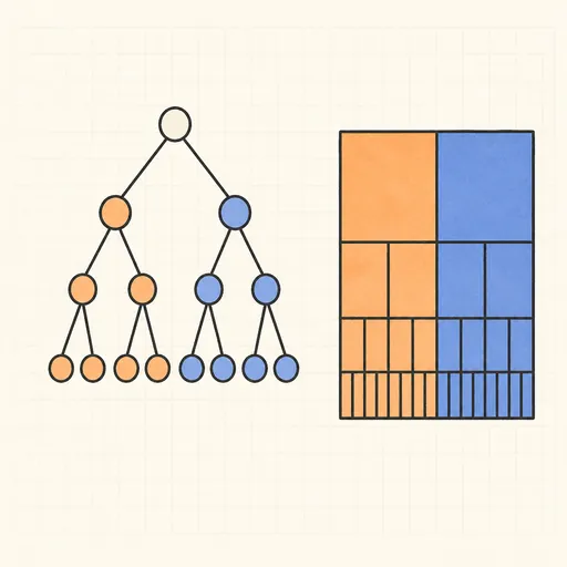
Grow a CART decision tree split by split and watch the partition map and tree diagram build together.