The Cross-Entropy Method on CartPole, Explained

After reading this you will understand how a four-number linear policy can balance an inverted pendulum, and how the cross-entropy method finds the weights for that policy by sampling, ranking and refitting a Gaussian, without ever computing a gradient.

What CartPole is and why it is the standard first problem

CartPole is a control task. A cart slides on a one-dimensional track. A pole is hinged to the top of the cart and can swing freely. At every time step you push the cart left or right with a fixed force, and the pole responds according to the physics of an inverted pendulum. The episode runs until the pole leans past 12 degrees from vertical, the cart leaves the track, or you reach 500 steps. The reward is one point per step, so the goal is simply to survive as long as possible.

The task earns its "fruit fly" reputation because it is small enough to reason about by hand yet hard enough to be interesting. The state is four numbers: cart position x, cart velocity \dot{x}, pole angle \theta, and pole angular velocity \omega. The action is binary: push left or push right. That is the entire interface.

Try Manual mode first. Even with only two buttons, keeping the pole up past 100 steps takes practice, because an inverted pendulum is unstable: a small tilt produces a torque that increases the tilt. Deviations grow roughly exponentially, so you have to push before the pole visibly falls, not after.

A linear policy is enough

You do not need a neural network here. A single weight vector solves CartPole. The policy takes the four state numbers, forms a weighted sum with a bias, and picks an action from the sign:

Here s = (x, \dot{x}, \theta, \omega) is the state, w is a vector of four weights, and b is a scalar bias. The dot product w \cdot s = w_1 x + w_2 \dot{x} + w_3 \theta + w_4 \omega collapses the four numbers into one, and the sign of that number plus the bias decides the push. Five numbers total: four weights and one bias.

Intuitively, a good policy weights the pole angle and angular velocity heavily. If the pole tilts right (\theta \gt 0) or is rotating right (\omega \gt 0), you want to push the cart right to slide back under the falling pole. So w_3 and w_4 should be positive and large. The cart position and velocity terms mostly keep the cart from drifting off the track.

The cross-entropy method as an optimizer

The cross-entropy method (CEM) does not follow a gradient. It treats the five policy numbers as a vector to be searched and maintains a Gaussian distribution over that vector. Each generation it samples candidate policies, scores them by episode length, keeps the best few, and refits the Gaussian to those survivors. Over generations the distribution concentrates around policies that balance well.

Formally, the parameter vector is \phi = (w_1, w_2, w_3, w_4, b), five numbers. The sampling distribution is a Gaussian with mean vector \mu and a diagonal covariance, so each coordinate i is drawn independently:

\mu_i is the current best guess for coordinate i, and \sigma_i is how far the method is willing to explore around it. The refit step is the whole idea. After scoring, you take the elite set (the top policies by episode length) and set the new mean and standard deviation to the sample mean and sample standard deviation of the elites:

Here K is the number of elites (6 in this demo) and \phi_i^{(k)} is coordinate i of the k-th elite. The mean moves toward what worked, and the standard deviation shrinks along any coordinate where the elites agree. That shrinking is what makes the method converge.

When to reach for it and when not to

CEM shines when the parameter space is small (tens of numbers), evaluations are cheap, and you have no gradient. That describes CartPole exactly: five parameters, an episode runs in milliseconds, and the reward is a step count with no usable derivative. The method is also easy to reason about and has almost no hyperparameters: population size, elite count, and an optional noise floor.

It scales poorly. With 1000 parameters you would need far more samples per generation to estimate the Gaussian, and the diagonal covariance ignores correlations between parameters. For large neural network policies, gradient-based methods such as policy gradients or PPO dominate. CEM is a fine baseline and a superb teaching tool, not a production solver for high-dimensional problems.

A worked run reproducing the demo defaults

The demo uses a population of 30 policies per generation, keeps the top 6 by episode length, and refits the Gaussian around them. The pole length and push force sliders stay at their defaults. Here is what one generation does, with small round numbers you can check.

Because each coordinate is refit independently, the same shrinking happens in parallel across all five numbers. Coordinates that matter (angle, angular velocity) converge to definite values; coordinates that barely affect survival keep a wider spread, which is fine because their exact value does not change the outcome.

Reading the learning curve

The tool plots two lines per generation: the best episode length and the mean episode length over the 30 sampled policies. Watch both. The best line tells you whether any policy in the population can balance; the mean line tells you whether the whole distribution has moved toward balancing. Early on the best line jumps around while the mean stays low. As the Gaussian concentrates, the mean climbs to meet the best, and both flatten at the 500-step cap.

A healthy run reaches 500 steps within a few dozen generations. If the best line stalls well below 500, the sampling distribution has probably collapsed too early onto a mediocre policy, which is the classic CEM failure discussed next.

Common mistakes and how to avoid them

The failures below are the ones that show up when people build or tune a CEM run themselves.

Premature collapse

If the standard deviation shrinks to near zero while the mean sits on a poor policy, every future sample is nearly identical and learning stops. In the worked example, sigma went from 0.50 to 0.1972 in one step. A few more such steps and it approaches zero. A small noise floor added to sigma each generation prevents this.

Too few elites

Keeping only 1 or 2 elites out of 30 makes the standard deviation estimate noisy and speeds collapse. The 6-of-30 default (20 percent) is a reasonable balance.

Evaluation noise

If the initial state is randomized, a lucky policy can post a long episode by chance and enter the elite set undeservedly. Averaging each policy over several episodes before ranking reduces this, at the cost of more computation.

Reacting instead of anticipating

This one bites you in Manual mode, not the trained policy. Because tilt grows exponentially, waiting until the pole visibly leans means the correction arrives too late. Push toward the direction the pole is already rotating, early.

Related tools on this site

CEM is one way to search for a policy. Two other reinforcement learning approaches on this site attack the problem differently. In Q-Learning Gridworld the agent learns a value for each state-action pair by trial and error and reads off the best path, rather than searching a space of whole policies. In Multi-Armed Bandit Lab you compare strategies for the pure exploration-versus-exploitation trade-off, which is the same tension you see when choosing the elite fraction and noise floor here.

Related tools

AI Learns to Drive (Neuroevolution)

Watch a population of neural-network cars evolve from crashing into corners to lapping a race track.

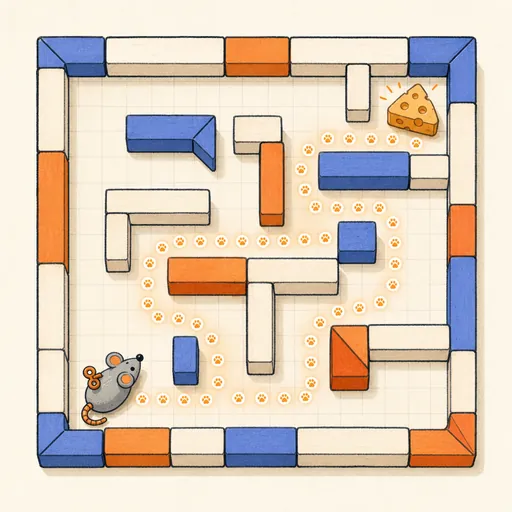
Q-Learning Gridworld

Paint a gridworld and watch a Q-learning agent discover the best path by trial and error.

Multi-Armed Bandit Lab

Race ε-greedy, UCB1 and Thompson sampling on the same bandit and compare their regret.

Backpropagation Step-by-Step

Walk through one forward and backward pass of a tiny neural network, number by number.

Decision Tree Builder

Grow a CART decision tree split by split and watch the partition map and tree diagram build together.

Diffusion Model Toy

Train a tiny denoising diffusion model and watch it turn pure noise back into a 2D shape.