Tail Latency and Autoscaling, Explained

After reading this you will understand why the 99th percentile of latency explodes as a service passes 80% utilization, why retries can collapse a system that was merely slow, and what an autoscaler can and cannot fix.

What tail latency is and one example

Latency is how long a request takes. The tail is the slowest few percent of those requests: p99 is the value that 99% of requests come in under, and p99.9 the value 99.9% come in under. Most users hit the median. The tail is where timeouts, angry customers and cascading failures live.

Here is the hook. Take a single worker that finishes 100 requests per second on average. Feed it 80 requests per second and the queue rarely builds up. The median wait is small and p99 sits maybe at three or four times the median. Now feed it 95 requests per second. The average worker is idle only 5% of the time, so any burst has almost no slack to recover into. The median barely moves, but p99 can jump by a factor of five or more. Utilization went up by 15 percentage points and the tail multiplied. That is the whole subject in one sentence.

The Tail Latency and Autoscaling Simulator makes this concrete: requests arrive as a random stream, wait in a queue, and are served by a pool of workers. It plots the p50, p95, p99 and p99.9 markers live so you can watch the tail pull away from the median.

When to reach for this model

Use queueing intuition whenever a shared resource serves independent arrivals: an HTTP service, a thread pool, a database connection pool, a disk. The three ingredients are an arrival process, a queue, and a finite number of servers. If those exist, the utilization-versus-tail curve applies.

Do not use it as a precise capacity forecast. Real systems have correlated arrivals, garbage collection pauses, cache effects and dependencies that break the independence assumptions. The formulas below give you the shape of the curve and the right order of magnitude, not a number you should paste into a spreadsheet and defend to four decimal places. Treat it as a way to reason, then measure your real system.

The formula and why the tail runs away

Let \lambda be the arrival rate (requests per second) and \mu the service rate of one server. Utilization for a single server is their ratio.

Here \rho is utilization, the fraction of time the server is busy. When \rho = 0.8 the server is busy 80% of the time. For the classic M/M/1 model (Poisson arrivals, exponential service times, one server), the average time a request spends waiting in the queue is:

The 1/\mu is the average service time. The dangerous factor is \rho / (1 - \rho). As \rho approaches 1, the denominator approaches 0 and the wait heads to infinity. That is the hockey stick.

Plug in numbers. At \rho = 0.5 the factor is 1.0. At \rho = 0.8 it is 4.0. At \rho = 0.95 it is 19.0. At \rho = 0.99 it is 99.0. Going from 50% to 80% quadruples the queue wait. Going from 80% to 95% multiplies it by nearly 5 again. Going from 95% to 99% multiplies it by another 5. Each equal-looking step up costs far more than the last.

Why the shape of service time matters

The formula above assumes exponential service times. Real workloads are often worse. A bimodal distribution, where 95% of requests take about 10 ms and 5% take about 100 ms, has a mean of 14.5 ms but a p99 near 100 ms. The mean barely notices the slow bucket; the tail is defined by it.

This is why fan-out amplifies pain. If one request calls 20 backend services in parallel and waits for all of them, the chance that every call avoids the slow 5% bucket is 0.95^{20} \approx 0.358. So about 64% of your fan-out requests hit at least one slow backend. A tail that affects 5% of single calls affects 64% of 20-way fan-outs. The p99 of the parent is driven by the p50-ish behavior of the children.

Retries, and how a slow service becomes a dead service

Now enable client timeouts and retries. This is where slowness turns into collapse. Suppose the client times out at 200 ms and retries once. Under light load few requests exceed 200 ms, so retries are rare. Under overload most requests exceed 200 ms, so almost every request generates a retry. Those retries are new arrivals.

Write it as a feedback loop. If a fraction f of requests time out and each retries once, the effective arrival rate becomes:

But higher \lambda_{\text{eff}} pushes utilization up, which raises latency, which raises f, which raises \lambda_{\text{eff}} again. Once \lambda_{\text{eff}} crosses total capacity, the queue grows without bound and served throughput falls even as the arrival count climbs. The system spends its time serving requests whose clients already gave up.

What the autoscaler can and cannot save

Turn on the autoscaler. It watches utilization and adds workers when utilization crosses a threshold. The catch is the warm-up delay: a new worker takes time to boot, connect and warm its caches before it serves traffic. Model that delay as D seconds.

During a sudden spike, the autoscaler cannot help for the first D seconds because the capacity you asked for does not exist yet. If a spike doubles arrivals and D = 60 seconds, you eat 60 seconds of overload latency no matter how good the scaling policy is. Capacity you must boot is not capacity you have.

The autoscaler is excellent against slow, predictable load changes such as a daily traffic ramp, where 60 seconds of lead time is invisible against a rise that takes 30 minutes. It is poor against instantaneous spikes and retry storms, because those move faster than D. Provisioning headroom (running at 60% rather than 90% baseline) buys you the slack to survive the warm-up window. That headroom is not waste; it is insurance priced in idle CPU.

Common mistakes when reasoning about latency

Watching the average instead of the tail

A mean of 20 ms can hide a p99 of 800 ms. Users experience the tail because they make many requests and remember the slow one. Alert on p99, not on the mean.

Targeting high utilization to save money

Running at 95% looks efficient on a cost dashboard. It means every burst turns into a latency spike, because there is no idle capacity to absorb it. The rho/(1-rho) factor at 95% is 19.0, nearly 5x the value at 80%.

Retrying without a budget or backoff

Retries feel safe under normal load and are lethal under overload. Cap them and add exponential backoff with jitter so retries spread out instead of arriving in a synchronized wave.

Assuming the autoscaler removes the need for headroom

The warm-up delay D means the autoscaler is always reacting to the past. Headroom covers the gap.

Related tools

Queueing sits next to several other systems topics on this site. The Cache Replacement Simulator shows how a hit-rate change moves your effective service time, which is the 1/\mu in the formula above. The Consistent Hashing Ring shows how load spreads across servers, deciding each server's \rho. The Raft Consensus Visualizer shows why a slow or partitioned replica raises tail latency for a whole cluster. For a different kind of runaway curve, the Regex Backtracking Visualizer shows a single request whose own service time explodes.

Related tools

Bloom Filter Playground

Add items, watch bits light up, measure the false positive rate.

Cache Replacement Simulator

Animate FIFO, LRU, LFU, CLOCK, ARC and Bélády's OPT on any access sequence.

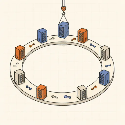
Consistent Hashing Ring

See why adding a server moves 1/N of the keys, not all of them.

Data Structure Visualizer

Watch BST, AVL, red-black trees, heaps, hash tables, tries and union-find work, step by step.

Digital Logic Gate Simulator

Build circuits from gates and flip-flops, wire them up, and watch the signals flow live.

Git Branching Sandbox

Type git commands and watch the commit DAG, branches and HEAD move — with levels, remotes, undo, and merge-vs-rebase contrast.