Z-Scores, Explained
After reading this you can turn any value into a z-score, read the percentile that goes with it, run the conversion backward from a percentile to a z, and find the probability that a normal variable lands between two z-scores.
What a z-score is
A z-score tells you how many standard deviations a value sits above or below the mean. If a test has a mean of 70 and a standard deviation of 5, then a score of 75 is one step of 5 above the mean, so its z-score is 1. A score of 80 is two steps above, so its z-score is 2. A score of 62.5 sits below the mean, so its z-score is negative: z = -1.5.
The point of the conversion is comparison on a common scale. Raw values carry their own units (points, kilograms, dollars). Z-scores strip the units away. A z-score of 1.5 means the same thing whether the raw variable was a height or a bank balance: the value is 1.5 standard deviations above average, which puts it near the 93rd percentile if the data are roughly normal.
When to use it and when not to
Z-scores are exact for the normal distribution and useful as a rough summary for any bell-shaped data. Use them to standardize a value, to compare scores from two different tests, or to look up a tail probability.
The percentile that a z-score maps to depends on the data being normal. For a z-score of 2, the normal model says the percentile is about 97.7. If your data are strongly skewed, that number can be far off. A right-skewed income distribution might put z = 2 at the 88th percentile instead. For skewed data, look at the Log-Normal calculator or the Gamma calculator instead.
A z-score is not a percentile. It becomes a percentile only through the normal cumulative distribution. The number 2 is a z-score; the number 97.7 is the percentile that goes with it under the normal model.
The formula and the intuition
To standardize a value, subtract the mean and divide by the standard deviation.
Here x is your value, \mu is the population mean, and \sigma is the population standard deviation. Subtracting \mu centers the value at zero. Dividing by \sigma rescales the distance into standard-deviation units.
To go from a z-score to a percentile, feed z into the standard normal cumulative distribution function \Phi. The percentile is 100 \cdot \Phi(z). To reverse the process and turn a percentile back into a z-score, use the inverse:
where p is the percentile from 0 to 100. And to recover the raw value from a z-score, rearrange the first formula: x = \mu + z\sigma. Those four moves (value to z, z to percentile, percentile to z, z to value) are the whole toolkit.
A worked example with the demo numbers
Standardizing a value of 75
Use the default inputs: value x = 75, mean μ = 70, standard deviation σ = 5.
- Subtract the mean:
75 - 70 = 5. - Divide by the standard deviation:
5 / 5 = 1. So z = 1. - Convert to a percentile with the normal CDF: \Phi(1) \approx 0.8413, so the value sits at about the 84.13th percentile.
Read that as: a score of 75 beats about 84% of the distribution. The remaining 15.87% score higher.
Now run the other demo modes. Setting the mode to Percentile from z with z = 1.5 gives \Phi(1.5) \approx 0.9332, the 93.32nd percentile. Setting the mode to z from a percentile with pct = 97.5 returns z \approx 1.960, the familiar cutoff behind a 95% confidence interval. Setting the mode to Area between two z-scores with z₁ = -1 and z₂ = 1 gives \Phi(1) - \Phi(-1) \approx 0.6827, the 68% covered by one standard deviation each side of the mean.
Explore how the tail area moves
Reading and interpreting the result
Match the number you get to the question you asked.
- z-score
- A signed count of standard deviations. Positive means above the mean, negative below. About 95% of normal data fall between
-1.96and1.96. - Percentile
- The share of the distribution at or below your value, times 100. A percentile of 84.13 means 84.13% score no higher.
- Area between two z-scores
- The probability of landing in a band. Between
-1and1that area is 0.6827; between-2and2it is 0.9545; between-3and3it is 0.9973.
| z | Left area (percentile) | Right tail |
|---|---|---|
| 0 | 0.5000 | 0.5000 |
| 1 | 0.8413 | 0.1587 |
| 1.645 | 0.9500 | 0.0500 |
| 1.960 | 0.9750 | 0.0250 |
| 2 | 0.9772 | 0.0228 |
| 3 | 0.9987 | 0.0013 |
Common mistakes
Confusing sample and population spread. The formula uses the population standard deviation \sigma. If you only have a sample and you estimate \sigma from it, the standardized value follows a t distribution, not a normal one, especially for small samples. Check the Student's t calculator when your sample is under about 30.
Dropping the sign. A value of 62.5 with mean 70 and \sigma = 5 has z = -1.5, not 1.5. The negative sign puts it at the 6.68th percentile, not the 93.32nd.
Reading a z-score as a probability. A z of 2 is not a 2% chance of anything. It becomes 0.0228 in the upper tail only after you apply \Phi.
Assuming normality without checking. The percentile lookup is only as good as the normal assumption. For counts, use the Poisson calculator or the Binomial calculator rather than forcing a z-score.
To sanity-check any percentile, compare it against the empirical rule: one standard deviation covers about 68%, two about 95%, three about 99.7%. If your z of 1 comes back as the 60th percentile, something is wrong with the inputs.
Related tools
The z-score is the standardized case of a general normal calculation. For arbitrary means and standard deviations without hand-standardizing, use the Normal Distribution calculator. To see where the 68-95-99.7 figures come from, try the Empirical Rule calculator. When you move to test statistics for variances or ratios of variances, the Chi-Square calculator and F Distribution calculator take over. For waiting times and other positive, skewed quantities, the Exponential calculator is a better fit.
Frequently asked questions
What is a good z-score?
There is no universally good value; it depends on context. In quality control a z-score near 0 (close to target) is desirable. On a standardized test, a higher z-score means a better relative result. A z of 1 puts you at the 84th percentile, a z of 2 at the 98th.
Can a z-score be greater than 3?
Yes, though it is rare in normal data. Only about 0.13% of values exceed z = 3 on the upper side. A z of 4 or more usually signals an outlier or a distribution that is not normal.
How do I convert a percentile back to a z-score?
Apply the inverse normal function. The 97.5th percentile gives z ≈ 1.960; the 90th gives z ≈ 1.282; the 50th gives z = 0. Set the mode to z from a percentile and enter the percentile directly.
Why is the standard normal mean 0 and standard deviation 1?
Standardizing subtracts the mean (which shifts the center to 0) and divides by the standard deviation (which rescales the spread to 1). Any normal distribution becomes this single reference curve after the transformation, so one table of areas serves every case.
What area lies between two z-scores?
Subtract the left areas: \Phi(z_2) - \Phi(z_1). Between -1 and 1 that is 0.8413 - 0.1587 = 0.6827. Use the Area between two z-scores mode to compute it directly.
Related tools
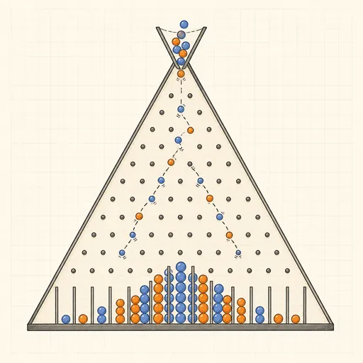
Binomial Distribution Calculator
Probabilities of k successes in n independent trials.
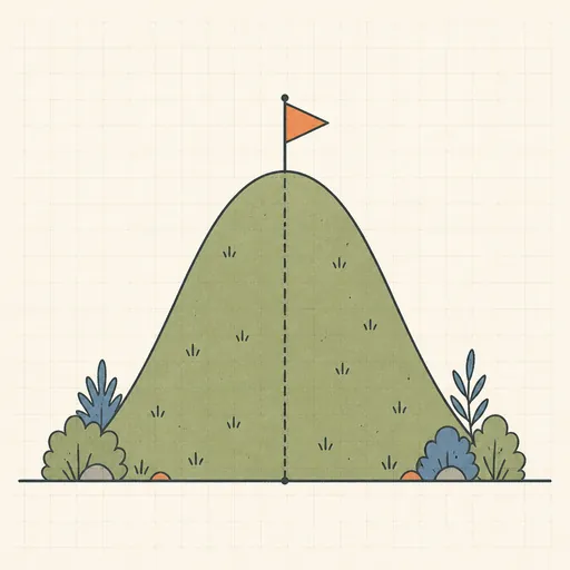
Normal Distribution Calculator
Probabilities, z-scores and inverse lookups for a normal distribution.

Poisson Distribution Calculator
PMF, CDF and tail probabilities for a Poisson distribution.
Chi-Square Distribution Calculator
p-values and critical values for the χ² distribution.

Empirical Rule (68-95-99.7) Calculator
Data ranges covered by 1, 2 and 3 standard deviations.

Exponential Distribution Calculator
Waiting-time probabilities for a Poisson process.