The Uniform Distribution, Explained
After reading this you will be able to compute densities, cumulative probabilities and quantiles for a continuous uniform distribution on any interval [a, b], and know when the model fits and when it does not.
What the uniform distribution is
The continuous uniform distribution spreads probability evenly across an interval [a, b]. Every value in that range is equally likely, and no value outside it can occur. Because the total area under a density must equal 1, and the interval has width b - a, the height of the density is the same everywhere: 1 / (b - a).
Here is a concrete hook. Suppose a bus arrives exactly every 10 minutes and you show up at a random moment without a schedule. Your waiting time is uniform on [0, 10]. The density is 1/10 = 0.1 per minute across the whole range. The chance you wait less than 7 minutes is the fraction of the interval below 7, which is 7/10 = 0.7. That single idea, probability equals fraction of the interval, drives everything below.
When to use it, and when not
Reach for the uniform model when you have a genuine reason to believe every outcome in a range is equally plausible and nothing outside the range can happen. Common cases:
- Rounding error. A value rounded to the nearest whole unit has a residual that is uniform on
[-0.5, 0.5]. - Arrival within a fixed window when you know nothing about timing, like the bus example.
- Random number generators. Most produce draws that are uniform on
[0, 1]before being transformed into other distributions.
Avoid it when the middle of the range is more likely than the edges. Heights of adults, measurement noise and sums of many small effects cluster near a center, so they call for the Normal calculator instead. Waiting times in a Poisson process are not uniform either; they follow the Exponential distribution. Proportions bounded on [0, 1] that are not flat belong to the Beta distribution.
A flat histogram is not proof of uniformity. Small samples from many distributions look roughly flat. Check that the support is genuinely bounded and that there is a mechanism forcing equal likelihood, not just a sample that happens to look level.
The formulas and the intuition
The probability density function (PDF) is constant inside the interval and zero outside:
Here a is the lower bound, b is the upper bound, and x is the value you are asking about. The density is a height, not a probability. For a continuous distribution the probability at a single point is 0; probability comes from area.
The cumulative distribution function (CDF) gives the probability of landing at or below x. It is the fraction of the interval to the left of x:
Below a it is 0; above b it is 1. To go the other way, from a probability p back to a value, invert the CDF. This gives the quantile function:
The mean sits at the midpoint and the variance depends only on the width:
For [0, 10] the mean is 5 and the variance is 100/12 \approx 8.333, so the standard deviation is \sqrt{8.333} \approx 2.887.
A worked example with the demo values
Waiting up to 7 minutes on [0, 10]
The demo uses a = 0, b = 10, x = 7 and p = 0.5. Work through the probability mode first.
- Confirm the interval width: b - a = 10 - 0 = 10.
- Density at any interior point, including
x = 7: f(7) = 1/10 = 0.1. - Cumulative probability at 7: F(7) = (7 - 0)/10 = 0.7. So P(X \le 7) = 0.7.
- Upper tail: P(X \gt 7) = 1 - 0.7 = 0.3.
Now the critical mode, going from probability to value. With p = 0.5:
- Apply the quantile formula: x = 0 + 0.5 \times 10 = 5.
- The 50th percentile is 5, which matches the mean because the uniform distribution is symmetric.
You can check any percentile the same way. The 90th percentile is 0 + 0.9 \times 10 = 9, and the 25th is 0 + 0.25 \times 10 = 2.5.
Explore how the bounds reshape the picture
Reading and interpreting results
Three numbers come out of this calculator. Keep them straight.
- Density f(x)
- A height, always 1/(b-a) inside the range. It can exceed 1 when the interval is narrow. On
[0, 0.5]the density is 2. That is fine; density is not probability. - Cumulative probability F(x)
- The area to the left of x, a number between 0 and 1. This is the probability that a draw falls at or below x.
- Quantile x(p)
- The value with probability p below it. The 0.5 quantile is the median, which equals the mean for a uniform distribution.
To find the probability of landing between two values c and d, subtract their cumulative probabilities. On [0, 10], P(3 \le X \le 8) = F(8) - F(3) = 0.8 - 0.3 = 0.5. Half the probability lies in the middle five units, exactly as the flat shape predicts.
Common mistakes
The uniform distribution is simple, which makes its errors easy to overlook.
- Treating density as probability. A density of 0.1 does not mean a 10 percent chance at that exact point. Point probabilities are 0. Use the CDF for probabilities.
- Swapping the bounds. If you enter
a = 10andb = 0, the width b - a goes negative and the formulas break. Always put the smaller number in a. - Asking about x outside the range. Any x \lt a has F(x) = 0, and any x \gt b has F(x) = 1. The density there is 0, not undefined.
- Confusing continuous with discrete uniform. Rolling a fair die is discrete uniform over six values, so each face has probability 1/6 \approx 0.1667. This calculator handles the continuous case, where probability comes from intervals, not single points.
The uniform on [0, 1] is the workhorse behind simulation. If U is uniform on [0, 1], then applying the inverse CDF of any distribution to U produces a draw from that distribution. That is why so many models start from a flat unit interval.
Related calculators
If your data cluster near a center rather than lying flat, the Normal distribution or the Z-Score calculator fit better. For waiting times in a Poisson process, use the Exponential distribution, and for the counts themselves the Poisson calculator. Bounded proportions that are not flat belong to the Beta distribution. For counts of successes in fixed trials, see the Binomial calculator. Right-skewed positive quantities are covered by the Gamma and Log-Normal calculators, and failure times by the Weibull calculator.
Frequently asked questions
Why can the uniform density be greater than 1?
Density is a height, and heights are unbounded as long as the total area is 1. On [0, 0.25] the density is 1/0.25 = 4. The area is still 4 \times 0.25 = 1, so it is a valid distribution.
What is the probability of an exact value?
Zero. For any continuous distribution, including this one, P(X = c) = 0. Probabilities only accumulate over intervals of positive width, so P(X \le 7) is meaningful but P(X = 7) is not.
How do I find the probability between two values?
Subtract the two cumulative probabilities: P(c \le X \le d) = (d - c)/(b - a). On [0, 10], the chance of landing between 4 and 6 is (6 - 4)/10 = 0.2.
What is the difference from a discrete uniform distribution?
A discrete uniform assigns equal probability to a finite list of values, like the six faces of a die at 1/6 each. The continuous version spreads probability over an entire interval and gives probabilities only for ranges. This page covers the continuous case.
How are the mean and standard deviation computed?
The mean is the midpoint, (a + b)/2. The variance is (b - a)^2 / 12, so the standard deviation is (b - a)/\sqrt{12}. For [0, 10] that is a mean of 5 and a standard deviation of about 2.887.
Related tools
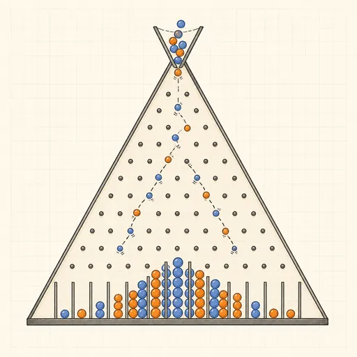
Binomial Distribution Calculator
Probabilities of k successes in n independent trials.
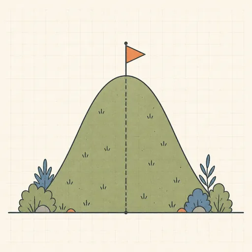
Normal Distribution Calculator
Probabilities, z-scores and inverse lookups for a normal distribution.

Poisson Distribution Calculator
PMF, CDF and tail probabilities for a Poisson distribution.
Z-Score Calculator
Convert between values, z-scores, percentiles and areas.
Chi-Square Distribution Calculator
p-values and critical values for the χ² distribution.

Empirical Rule (68-95-99.7) Calculator
Data ranges covered by 1, 2 and 3 standard deviations.