Regression Metrics, Explained
After reading this you will know how to compute MSE, RMSE, MAE, MAPE and R² by hand, and how to pick the metric that answers your actual question about a set of predictions.
What these metrics measure
You have two columns of numbers: the actual values you observed and the values a model predicted. Regression metrics turn the gap between those columns into a single number so you can compare models or track improvement.
Consider five predictions. Actual: 3, 5, 7, 9, 11. Predicted: 2.8, 5.3, 6.6, 9.4, 10.9. The errors (actual minus predicted) are 0.2, -0.3, 0.4, -0.4, 0.1. Each metric summarizes those five residuals in a different way. Mean absolute error reports the typical size of a miss (0.28 here). Root mean squared error weights the larger misses more heavily (0.30 here). R² asks how much of the variation in the actuals your predictions explained (0.984 here). None of these is "the" answer. Each answers a specific question.
When to use each metric, and when not to
Choose the metric that matches the cost of being wrong.
- MAE (mean absolute error)
- Use when every unit of error costs the same. A forecast off by 10 is twice as bad as one off by 5. Robust to outliers.
- RMSE (root mean squared error)
- Use when large errors are disproportionately costly. Squaring makes a single big miss dominate. Sensitive to outliers.
- MAPE (mean absolute percentage error)
- Use when errors should be judged relative to the size of each value. Being off by 5 on a value of 10 (50%) is worse than off by 5 on a value of 1000 (0.5%).
- R² (coefficient of determination)
- Use to compare against the naive baseline of always guessing the mean. Unitless, so it travels across problems.
Do not use MAPE when any actual value is zero or near zero. Dividing by zero is undefined, and dividing by 0.01 produces a percentage in the thousands that swamps every other term. If your actuals cross zero, use MAE or RMSE instead.
The formulas and the intuition
Write y_i for the actual value and \hat{y}_i for the prediction, with n pairs.
Mean squared error averages the squared residuals. Squaring removes the sign and punishes big errors: a residual of 2 contributes 4, but a residual of 4 contributes 16. The units are the square of your data's units, which makes MSE hard to interpret directly.
Taking the square root returns you to the original units. If your actuals are in dollars, RMSE is in dollars. Because of the squaring inside, RMSE is always greater than or equal to MAE, and the two are equal only when every error has the same magnitude.
Mean absolute error averages the absolute residuals. It is the plain answer to "how far off am I on average," in the original units, with no extra weight on outliers.
Mean absolute percentage error scales each residual by its own actual value, then averages. The result is a percentage that carries no units at all.
Here \bar{y} is the mean of the actuals. The numerator is the sum of squared errors from your model. The denominator is the sum of squared errors from always guessing \bar{y}. If your model matches that baseline exactly, the ratio is 1 and R² is 0. If your model is perfect, the numerator is 0 and R² is 1. A model worse than the mean gives a negative R².
A worked example with the demo data
Five predictions, all five metrics
Actual: 3, 5, 7, 9, 11. Predicted: 2.8, 5.3, 6.6, 9.4, 10.9.
- Residuals y_i - \hat{y}_i:
0.2, -0.3, 0.4, -0.4, 0.1. - Squared residuals:
0.04, 0.09, 0.16, 0.16, 0.01. Sum =0.46. - MSE =
0.46 / 5 = 0.092. - RMSE = \sqrt{0.092} \approx 0.3033.
- Absolute residuals:
0.2, 0.3, 0.4, 0.4, 0.1. Sum =1.4. MAE =1.4 / 5 = 0.28. - Percentage errors:
6.67%, 6.00%, 5.71%, 4.44%, 0.91%. Sum =23.73%. MAPE =23.73 / 5 = 4.75%. - Mean of actuals \bar{y} = 7. Deviations from mean:
-4, -2, 0, 2, 4. Squared:16, 4, 0, 4, 16. Sum =40. - R² = 1 - 0.46 / 40 = 0.9885.
So the predictions miss by about 0.28 on average (MAE), the RMSE of 0.30 is only a touch larger because no single error dominates, the typical relative miss is under 5% (MAPE), and the model explains 98.85% of the variation in the actuals (R²).
How an outlier splits RMSE from MAE
MAE and RMSE agree closely when errors are similar in size, as in the demo. They diverge when one error is large. Suppose four predictions are perfect and the fifth misses by 10. The absolute errors are 0, 0, 0, 0, 10. MAE = 10 / 5 = 2. But the squared errors are 0, 0, 0, 0, 100, so MSE = 100 / 5 = 20 and RMSE = \sqrt{20} \approx 4.47. The RMSE is more than twice the MAE, flagging that the average hides one bad miss. Watch the gap between the two: a large ratio of RMSE to MAE means your errors are uneven.
Reading and interpreting the results
Read every metric next to the scale of your data. An RMSE of 0.30 is excellent if your actuals run from 3 to 11, and terrible if they run from 0 to 1. R² fixes the scale problem by construction, which is why it is the easiest single number to report across different datasets.
Some rules of thumb worth keeping:
- R² of 1.0 means perfect predictions. R² of 0.0 means you did no better than guessing the mean. Negative R² means you did worse than the mean.
- RMSE is always at least as large as MAE. If they are nearly equal, your errors are uniform.
- MAPE below 10% is often called accurate in demand forecasting, but the threshold depends entirely on the field.
Report at least two metrics. RMSE plus R² is a common pair: RMSE gives error in real units, R² gives the fit relative to the baseline. A model can have a low RMSE simply because the values themselves barely vary, and R² will expose that.
Common mistakes
Comparing R² across different target variables. R² is relative to each dataset's own variance. An R² of 0.7 on one problem is not automatically better than 0.6 on another.
Chasing R² on the training data. Adding more predictors never lowers R² on the data you fit, even when the predictors are noise. Judge a model on data it has not seen.
Mismatched or reversed columns. Every metric here except R² is symmetric in a subtle way: MSE, RMSE and MAE give the same value if you swap actual and predicted, but MAPE and R² do not, because they divide by the actuals or the actual mean. Keep the columns in the right order.
Averaging percentages when values cross zero. As noted, MAPE explodes near zero. It also treats over-prediction and under-prediction asymmetrically, since the denominator is always the actual value.
Related calculators
To fit the line or curve that produces these predictions, start with the Correlation and Linear Regression Calculator for a straight-line fit with Pearson r and R², or the Polynomial Regression Calculator when the relationship bends. For classification problems, where the target is a category rather than a number, these error metrics do not apply; use the Confusion Matrix Metrics Calculator for accuracy, precision, recall and F1 instead.
Frequently asked questions
Which metric is best for regression?
There is no single best metric. Use MAE when all errors cost the same, RMSE when big errors cost disproportionately more, MAPE when relative error matters, and R² to compare against a mean baseline. Reporting two or three together tells a fuller story.
Why is my RMSE larger than my MAE?
RMSE is always greater than or equal to MAE. Squaring inside RMSE inflates larger errors before averaging, so the gap widens when your errors are uneven. In the demo data RMSE is 0.30 and MAE is 0.28, a small gap that reflects similar error sizes.
Can R² be negative?
Yes. R² is negative when your predictions have a larger squared error than simply predicting the mean of the actuals. It signals a model that is actively harmful, not just weak.
What is a good MAPE?
It depends on the field. In stable demand forecasting a MAPE under 10% is often treated as accurate, but volatile series may never beat 30%. Compare against a naive forecast rather than a fixed threshold.
Do these metrics need equal-length columns?
Yes. Each metric pairs the i-th actual with the i-th prediction, so the two columns must have the same length and the same ordering. A mismatch produces meaningless numbers.
Related tools

Correlation & Linear Regression Calculator
Pearson r, Spearman ρ, R² and the least-squares line.

Confusion Matrix Metrics Calculator
Accuracy, precision, recall, F1, MCC and more from TP/FP/FN/TN.
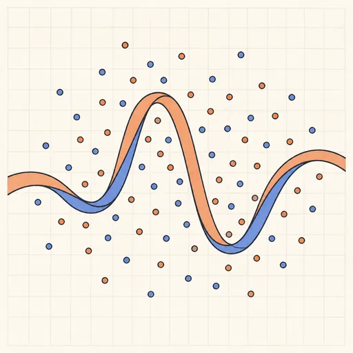
Polynomial Regression Calculator
Fit a polynomial of degree 2–8 with R² and residuals.
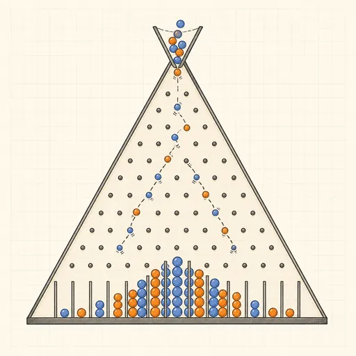
Binomial Distribution Calculator
Probabilities of k successes in n independent trials.

Chi-Square Test of Independence
Test association between two categorical variables from a contingency table.

Combinations & Permutations Calculator
nCr and nPr, with and without repetition.