Queueing Theory, Explained
After reading this you can compute how long a line will be, how long each customer waits, and how many servers you need to keep both under control, using the M/M/1 and M/M/c models.
What queueing theory computes
A queue forms whenever work arrives faster than it can be served, even briefly. Queueing theory turns two numbers, the arrival rate and the service rate, into the metrics you actually care about: the average number of customers in the system, the average time each one spends waiting, and how often the system sits idle.
Here is the hook. Suppose customers arrive at a help desk at 4 per hour, and one agent handles 5 per hour. The agent is busy only 80% of the time, so you might expect short lines. Instead the average number of customers in the system is 4, and each customer spends a full hour there on average. The idle 20% is not slack you can rely on, because arrivals and service times both vary.
The models here assume Poisson arrivals and exponential service times. That is what the two "M" letters mean (Markovian). M/M/1 has one server; M/M/c has c identical servers sharing one queue.
When to use these models, and when not
Use M/M/1 or M/M/c when arrivals are independent and roughly random in time, service times vary a lot, and there is a single waiting line. Call centers, checkout counters with one shared queue, and packet routers all fit reasonably well.
Be careful in three situations. First, if customers arrive in scheduled batches (a factory shipping dock), arrivals are not Poisson and the formulas overstate variability. Second, if service times are nearly constant, the real waiting time is about half what M/M/1 predicts. Third, if the queue has a hard capacity limit or customers leave when the line is long, you need a different model.
The single most important check is stability. The system reaches a steady state only when \rho = \lambda / (c\mu) \lt 1. If arrivals meet or exceed capacity, the queue grows without bound and every "average" below is infinite. The calculator will flag this.
The formulas and the intuition
Start with utilization, the fraction of server capacity in use:
Here \lambda is the arrival rate, \mu is the service rate per server, and c is the number of servers. With \lambda = 4, \mu = 5, and c = 1, utilization is 0.8.
The engine of interpretation is Little's law, which links the average number in the system L to the average time in the system W:
This is bookkeeping, not statistics. It holds for any stable queue regardless of the arrival or service distribution. If 4 customers arrive per hour and each spends 1 hour in the system, then on average 4 customers are present. That is all the law says, and it is always true.
For M/M/1 the average number in the system has a clean closed form:
Notice the 1 - \rho in the denominator. As \rho climbs toward 1, L blows up. At \rho = 0.5, L = 1. At \rho = 0.9, L = 9. At \rho = 0.99, L = 99. Small increases in load near full utilization cause enormous increases in the line.
For M/M/c the wait depends on the probability that an arriving customer finds all c servers busy. That quantity is the Erlang C formula:
The sum runs over the states with an idle server. Once you have P_{wait}, the average waiting time in queue is W_q = P_{wait} / (c\mu - \lambda), and the rest follows from Little's law. The calculator handles the sum for you.
A worked example with the demo numbers
One server, λ = 4, μ = 5
These are the demo values. Load them and press Calculate to reproduce every number below.
- Utilization: \rho = 4/5 = 0.8. The server is busy 80% of the time.
- Probability of an empty system: P_0 = 1 - \rho = 0.2. One visit in five finds no one there.
- Number in system: L = 0.8 / (1 - 0.8) = 4 customers.
- Time in system, from Little's law: W = L / \lambda = 4 / 4 = 1 hour.
- Number waiting in line (excluding the one being served): L_q = \rho \cdot L = 0.8 \times 4 = 3.2 customers.
- Time spent waiting before service: W_q = L_q / \lambda = 3.2 / 4 = 0.8 hours, that is 48 minutes.
The service itself takes 1/\mu = 0.2 hours (12 minutes), and 48 + 12 = 60 minutes matches W = 1 hour. The arithmetic closes.
How the numbers explode near full load
The table shows M/M/1 with \mu = 5 fixed while \lambda rises. Watch the last three rows.
| λ | ρ | L (in system) | L_q (waiting) | W (hours) |
|---|---|---|---|---|
| 2.5 | 0.5 | 1 | 0.5 | 0.4 |
| 4.0 | 0.8 | 4 | 3.2 | 1.0 |
| 4.5 | 0.9 | 9 | 8.1 | 2.0 |
| 4.75 | 0.95 | 19 | 18.05 | 4.0 |
| 4.9 | 0.98 | 49 | 48.02 | 10.0 |
Reading and interpreting the results
- Utilization ρ
- Fraction of capacity in use. Aim to keep it below about 0.85 for one server if you want predictable waits. Above 0.9 the queue is fragile.
- P₀
- Probability the system is completely empty. For M/M/1 it equals 1 - \rho. A small P₀ means customers rarely walk into an open server.
- L and L_q
- Average number in the system and average number waiting. They differ by the number in service, which averages c\rho.
- W and W_q
- Average time in the system and average time waiting before service. W = W_q + 1/\mu.
- P_wait (Erlang C)
- Probability an arriving customer must wait at all. In staffing this is the target: a call center might size c so that P_{wait} \le 0.2.
Common mistakes
Reading averages as guarantees. An average wait of 48 minutes does not mean everyone waits 48 minutes. In M/M/1 the waiting time is highly variable; some customers walk straight to the server while others wait far longer than the mean.
Confusing L with L_q. The line you see is L_q, the people waiting. The person at the counter is in the system but not in the queue. In the demo, L = 4 but L_q = 3.2.
Comparing rates in different units. If λ is per hour, μ must be per hour too. Mixing per-minute and per-hour rates is the most frequent error.
Treating c servers as one fast server. Two servers at μ = 5 each are not the same as one server at μ = 10. Two servers can leave one idle while a job waits; a single fast server never does. The M/M/c and M/M/1 numbers differ, and the calculator keeps them separate.
Related tools
Queueing rests on the Poisson and exponential distributions, both built from independent random events. To combine such events or compute an at-least-once probability, use the Probability Calculator. To find the mean and variance of a discrete outcome such as queue length, the Expected Value Calculator does the arithmetic. If you are updating a belief from evidence rather than modeling flow, see the Bayes' Theorem Calculator.
Frequently asked questions
What is the difference between M/M/1 and M/M/c?
Both share one waiting line and Poisson arrivals with exponential service. M/M/1 has a single server; M/M/c has c identical servers. With c = 1 the M/M/c formulas reduce exactly to M/M/1.
Why does the wait explode as utilization nears 100%?
Because of the 1 - \rho in the denominator of L = \rho/(1-\rho). At \rho = 0.9, L = 9; at 0.99, L = 99. Variability in arrivals and service means the last sliver of capacity gets swamped by random bursts.
Does Little's law really need no distribution assumptions?
Yes. L = \lambda W holds for any stable system in steady state, whatever the arrival or service pattern. It is a conservation identity. Only the closed forms for L (like \rho/(1-\rho)) depend on the M/M assumptions.
What if my arrivals are scheduled, not random?
Then M/M overstates the wait. Scheduled or regular arrivals have less variability than Poisson, so real queues are shorter. Treat these results as a conservative upper bound.
How many servers do I need?
Pick a target, such as P_wait below 0.1 or W_q below 5 minutes, then raise c in the calculator until the metric drops under your target. Because of the Erlang C shape, one extra server near a busy threshold often cuts the wait by more than half.
Related tools
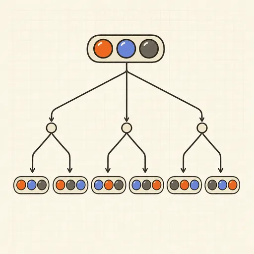
Combinations & Permutations Calculator
nCr and nPr, with and without repetition.

Bayes' Theorem Calculator
Posterior probabilities, plus a diagnostic-test mode (PPV, NPV, LRs).
Dice Probability Calculator
Exact sum probabilities for any number of dice.
Expected Value Calculator
E[X], variance and SD of a discrete distribution.
Probability Calculator
Combine independent events, conditional and at-least-once probabilities.

Birthday Paradox Calculator
Probability that two people in a group share a birthday.