The Normal Distribution, Explained
After reading this you can turn any value into a probability, turn any probability back into a value, and know when the normal model is the right one.
The normal distribution is the smooth, symmetric bell curve that shows up whenever many small independent effects add together: measurement error, adult heights, the average of a large sample. It has two parameters. The mean \mu sets the center, and the standard deviation \sigma sets the spread. Every question you ask reduces to one of two tasks: find the probability that falls below a value, or find the value that sits below a given probability.
Here is the hook. Adult resting heart rate is roughly normal with mean 70 beats per minute and standard deviation 10. What fraction of people beat below 90? That is z = (90 - 70) / 10 = 2, and the area below z = 2 is about 0.9772. So about 97.7% fall below 90 bpm, and 2.3% above. You did not need a table for the shape, only for the standard normal.
What the distribution describes
The normal distribution assigns a density to every real number from -\infty to +\infty. The density is highest at the mean and drops off symmetrically. Because it is continuous, the probability of any single exact value is zero; only intervals carry probability. When you ask "what is the chance x is below 90," you are measuring the area under the curve to the left of 90.
Three anchor facts describe the spread. About 68% of the area sits within one standard deviation of the mean, about 95% within two, and about 99.7% within three. For heart rate with \mu = 70 and \sigma = 10, that means 68% fall between 60 and 80, and 95% between 50 and 90. The Empirical Rule calculator works these ranges out directly.
The precise two-sided 95% range uses z = 1.96, not 2. So 95% of heart rates fall between 70 - 1.96(10) = 50.4 and 70 + 1.96(10) = 89.6. The "2" in the empirical rule is a rounded teaching number.
When to use it, and when not to
The normal model fits data that is roughly symmetric and unbounded in both directions, especially averages and sums. The central limit theorem is the reason: the mean of many independent observations tends toward a normal shape even when the raw data is not normal.
It is the wrong model in several common cases. Counts of events per interval follow the Poisson distribution. Successes in a fixed number of trials follow the Binomial distribution. Right-skewed quantities like incomes or file sizes are better described by the Log-Normal distribution, and waiting times by the Exponential distribution. If your data cannot go below zero and piles up near it, do not force a symmetric bell onto it.
When you estimate \sigma from a small sample rather than knowing it, use the Student's t distribution, which has heavier tails.
The formula and the intuition
The probability density function is
The term (x-\mu)^2 is the squared distance from the center, so density falls off fast as you move away. Dividing by 2\sigma^2 scales that distance by the spread: a large \sigma makes the curve wide and low, a small one makes it tall and narrow. The leading fraction keeps the total area equal to 1.
For probabilities you need the cumulative distribution function F(x), the area to the left of x. There is no elementary formula for it, so it is computed numerically through the standard normal CDF written \Phi(z). The bridge is the z-score:
The z-score counts how many standard deviations x lies above the mean. Once you have it, F(x) = \Phi(z). The inverse mode runs this backward: given a probability p, it finds the quantile
where \Phi^{-1} is the inverse standard normal, sometimes called the probit or quantile function. The Z-Score calculator handles the standardization step on its own if that is all you need.
A worked example with the demo data
Probability from a value on the standard normal
The demo uses the defaults: \mu = 0, \sigma = 1, and x = 1.96 in probability mode. This is the standard normal, so the z-score equals x.
- Standardize: z = (1.96 - 0) / 1 = 1.96.
- Look up the cumulative area: \Phi(1.96) \approx 0.9750.
- Interpret it: about 97.5% of the distribution lies below 1.96, and 2.5% lies above.
Now run the inverse to confirm it round-trips. Switch to inverse mode with p = 0.975, keeping \mu = 0 and \sigma = 1. The calculator returns x = 0 + 1 \cdot \Phi^{-1}(0.975) \approx 1.96. The value 1.96 and the probability 0.975 are two views of the same point. This is exactly why 1.96 is the critical value for a two-sided 95% confidence interval: 2.5% is cut off in each tail.
Reading and interpreting the output
The probability mode returns the cumulative area to the left of your value, F(x). To answer other questions, combine it:
- Left tail
- Probability below
xis F(x) directly. For the heart-rate example, F(90) = 0.9772. - Right tail
- Probability above
xis 1 - F(x). Above 90 bpm:1 - 0.9772 = 0.0228. - Between two values
- Probability between
aandbis F(b) - F(a). Between 60 and 80: F(80) - F(60) = 0.8413 - 0.1587 = 0.6826, the familiar 68%.
The inverse mode returns a value on the original scale, already unstandardized. Ask for the 90th percentile of heart rate with \mu = 70, \sigma = 10: \Phi^{-1}(0.90) \approx 1.2816, so x = 70 + 10(1.2816) = 82.8 bpm. Ninety percent of people fall below about 83.
| z | Left area Φ(z) | Right area | Two-sided outside |
|---|---|---|---|
| 1.000 | 0.8413 | 0.1587 | 0.3173 |
| 1.282 | 0.9000 | 0.1000 | 0.2000 |
| 1.645 | 0.9500 | 0.0500 | 0.1000 |
| 1.960 | 0.9750 | 0.0250 | 0.0500 |
| 2.576 | 0.9951 | 0.0049 | 0.0100 |
Common mistakes
Watch for these before you trust a result.
Do not confuse the standard deviation with the variance. The formula and the calculator take \sigma, not \sigma^2. If a source reports a variance of 25, enter 5, not 25. Entering the variance quintuples the spread here and turns a 95% range of 50 to 90 into 20 to 120.
A second error is confusing left and right tails. The calculator gives the left area. For an upper-tail p-value, subtract from 1. For heart rate above 90, the answer is 0.0228, not 0.9772.
A third is forgetting to unstandardize. If you compute \Phi^{-1}(0.975) = 1.96 but your data has \mu = 70 and \sigma = 10, the 97.5th percentile is 70 + 10(1.96) = 89.6, not 1.96. The inverse mode does this for you when you supply the real \mu and \sigma.
Finally, do not apply the normal model to bounded or skewed data. Reaction times, insurance claims, and particle counts have hard floors at zero and long right tails. Fitting a symmetric curve will predict impossible negative values and understate the extremes.
Related calculators
For discrete count models, see the Geometric, Negative Binomial, and Hypergeometric calculators. For continuous alternatives, the Uniform, Weibull, Gamma, and Beta calculators cover flat, reliability, waiting-time, and proportion data. For test statistics, the Chi-Square and F distribution calculators handle variance and analysis-of-variance work.
Frequently asked questions
What is the difference between the PDF and the CDF?
The PDF f(x) is the height of the curve at a point; it is not a probability. The CDF F(x) is the area to the left of x, which is a probability between 0 and 1. At z = 0 the PDF height is about 0.399 but the CDF is exactly 0.5.
Why is the probability of an exact value zero?
For a continuous distribution, probability is area, and a single point has zero width, so it has zero area. Only intervals carry probability. Ask for the chance between 89.5 and 90.5 instead of exactly 90 if you need a nonzero answer.
How do I get a two-sided probability?
For a symmetric range around the mean, the area outside \pm z is 2(1 - \Phi(z)). At z = 1.96 that is 2(1 - 0.975) = 0.05, the 5% behind a two-sided 95% interval.
What z-score matches a 95% confidence interval?
Use 1.96 for a two-sided 95% interval, since 2.5% falls in each tail. For a one-sided 95% bound use 1.645. For 99% two-sided use 2.576.
Can the mean be negative?
Yes. The mean can be any real number and shifts the whole curve left or right. Temperature anomalies and standardized scores routinely have negative means. Only the standard deviation must be positive.
Related tools
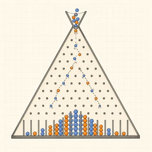
Binomial Distribution Calculator
Probabilities of k successes in n independent trials.

Poisson Distribution Calculator
PMF, CDF and tail probabilities for a Poisson distribution.
Z-Score Calculator
Convert between values, z-scores, percentiles and areas.
Chi-Square Distribution Calculator
p-values and critical values for the χ² distribution.

Empirical Rule (68-95-99.7) Calculator
Data ranges covered by 1, 2 and 3 standard deviations.

Exponential Distribution Calculator
Waiting-time probabilities for a Poisson process.