The Empirical Rule (68-95-99.7), Explained
After reading this you can take any normal distribution, given its mean and standard deviation, and state the value ranges that hold roughly 68%, 95% and 99.7% of the data.
What the rule says
The empirical rule is a quick summary of how data spreads out around the mean in a normal (bell-shaped) distribution. It tells you three things at once:
- About 68% of values fall within 1 standard deviation of the mean.
- About 95% fall within 2 standard deviations.
- About 99.7% fall within 3 standard deviations.
Take IQ scores, which are built to have a mean of 100 and a standard deviation of 15. The rule says about 68% of people score between 85 and 115, about 95% score between 70 and 130, and about 99.7% score between 55 and 145. Those are the calculator's default inputs, and the rest of this article reproduces them.
The name comes from the three percentages, and "empirical" reflects that these numbers describe what you actually observe in real normal data, not just theory.
When to use it, and when not to
The rule is a fast mental check. Use it when you already know the mean and standard deviation and you want the range that covers a familiar fraction of the data, or when you want to spot whether a value is unusual. A score 3 standard deviations above the mean sits past the 99.7% band, so it is rarer than 1 in 300.
The rule only holds for distributions that are roughly normal: symmetric, single peaked, with thin tails. It fails for skewed data. Household income, for example, has a long right tail, so far less than 68% sits within one standard deviation of the mean. For skewed positive quantities look at the Log-Normal calculator or the Gamma calculator instead.
The empirical rule is an approximation for normal data only. If your data are counts, waiting times or proportions, a normal shape may not apply at all. Check a histogram before you trust the 68-95-99.7 split.
The formula and the intuition
The three ranges come from adding and subtracting multiples of the standard deviation from the mean:
Here \mu is the mean, \sigma is the standard deviation, and k is the number of standard deviations. The interval \mu \pm 1\sigma runs from \mu - \sigma to \mu + \sigma.
The percentages themselves come from the area under the normal curve. The exact areas are 68.27%, 95.45% and 99.73%, which round to the familiar 68, 95 and 99.7. If you want the exact area for any interval, not just whole multiples of \sigma, use the Normal distribution calculator.
One useful way to read the rule: the middle 68% band leaves 32% in the two tails combined, so each tail holds about 16%. The 95% band leaves 5% total, about 2.5% per tail. The 99.7% band leaves 0.3%, about 0.15% per tail.
Worked example with the default data
IQ scores: mean 100, standard deviation 15
Set \mu = 100 and \sigma = 15, then apply \mu \pm k\sigma for each k.
- One standard deviation:
100 - 15 = 85and100 + 15 = 115. Range85to115, about 68%. - Two standard deviations:
100 - 30 = 70and100 + 30 = 130. Range70to130, about 95%. - Three standard deviations:
100 - 45 = 55and100 + 45 = 145. Range55to145, about 99.7%.
You can also read the bands the other way. The share of scores between 115 and 130 (that is, between 1 and 2 standard deviations above the mean) is half of the difference between 95% and 68%, which is (95 - 68) / 2 = 13.5%.
| Standard deviations | Lower | Upper | Approx. share inside | Approx. share outside |
|---|---|---|---|---|
| ±1σ | 85 | 115 | 68% | 32% |
| ±2σ | 70 | 130 | 95% | 5% |
| ±3σ | 55 | 145 | 99.7% | 0.3% |
Explore the bands
Reading and interpreting the results
The bands answer two directions of question. Given a range, what fraction sits inside? Given a fraction, what range holds it? Both come from the same three lines.
To judge whether a single value is unusual, count how many standard deviations it sits from the mean. An IQ of 130 is (130 - 100) / 15 = 2 standard deviations above the mean. That is the edge of the 95% band, so only about 2.5% of people score higher. This count is the z-score, and the Z-Score calculator turns it into an exact percentile.
Be careful with one-sided versus two-sided language. The 95% band is two-sided: 95% inside, 2.5% below 70 and 2.5% above 130. If someone asks for the fraction above a single cutoff, you want one tail, not the whole 5%.
Common mistakes
Applying it to skewed data. A right-skewed variable can have far more than 16% of its mass in the upper tail past \mu + \sigma. The rule reports the wrong split. Confirm approximate symmetry first.
Confusing 95% with two standard deviations exactly. The 95% figure is a rounding of 95.45%, which comes from exactly 2σ. The clean 95% confidence bound many people cite uses 1.96 standard deviations, not 2. For a quick range use 2; for a reported interval use 1.96.
Reading percentages as counts. With a sample of 40 observations, "68%" does not guarantee 27 or 28 fall in the band. The rule describes the underlying distribution, and small samples wobble around it.
To sanity-check any band, remember that each step out adds a shrinking slice: 0 to 1σ holds about 34% per side, 1σ to 2σ adds about 13.5%, and 2σ to 3σ adds only about 2.35%. Almost everything is within 2σ.
Related calculators
The empirical rule is the fast approximation. For exact work, reach for the full normal tools. The Normal distribution calculator gives the area for any interval and any bound. The Z-Score calculator converts values to standard-deviation counts and percentiles.
When the normal shape does not fit, other distributions apply. Use the Binomial calculator for counts of successes, the Poisson calculator for event counts over an interval, and the Exponential calculator for waiting times. For small-sample means where \sigma is estimated, the Student's t calculator is the right choice, and variance tests use the Chi-Square calculator and the F distribution calculator.
Frequently asked questions
Why is it called the 68-95-99.7 rule?
Those are the approximate percentages of normal data within 1, 2 and 3 standard deviations of the mean. The exact areas are 68.27%, 95.45% and 99.73%.
Does the empirical rule work for any data?
No. It holds only for roughly normal, bell-shaped data. For skewed distributions the percentages are wrong. As a much weaker fallback for any distribution, Chebyshev's inequality guarantees at least 75% within 2σ and about 88.9% within 3σ.
What is the difference between 2σ and the 95% confidence value?
Exactly 2σ captures 95.45% of a normal distribution. The value that captures exactly 95% is 1.96σ. The empirical rule rounds 1.96 to 2 for convenience.
How do I find the percentage between two values that are not whole standard deviations apart?
The empirical rule only handles multiples of 1, 2 and 3. For any other cutoff, convert each value to a z-score and use the Normal distribution calculator for the exact area.
What fraction lies beyond 3 standard deviations?
About 0.3% total, split as roughly 0.15% in each tail. A value past 3σ is rarer than about 1 in 300.
Related tools
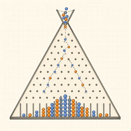
Binomial Distribution Calculator
Probabilities of k successes in n independent trials.
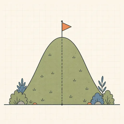
Normal Distribution Calculator
Probabilities, z-scores and inverse lookups for a normal distribution.

Poisson Distribution Calculator
PMF, CDF and tail probabilities for a Poisson distribution.
Z-Score Calculator
Convert between values, z-scores, percentiles and areas.
Chi-Square Distribution Calculator
p-values and critical values for the χ² distribution.

Exponential Distribution Calculator
Waiting-time probabilities for a Poisson process.