Bayes' Theorem, Explained
After reading this you can update a prior probability with new evidence, and read a diagnostic test correctly using prevalence, sensitivity and specificity.
What Bayes' theorem does
Bayes' theorem takes a probability you believe before seeing evidence, then revises it once the evidence arrives. The starting belief is the prior. The revised belief is the posterior.
Here is the hook. Suppose a disease affects 1 in 100 people. A test catches 90% of true cases and gives a false alarm only 5% of the time. You test positive. Your gut says the chance you are sick is near 90%. The correct answer is about 15%. That gap is why this calculator exists, and the rest of this article shows exactly where the 15% comes from.
When to use it, and when not
Use Bayes' theorem whenever you have a base rate and a piece of evidence whose reliability you can quantify. Medical screening is the classic case, but the same math handles spam filtering, quality control and any "given a signal, what is the true state" question.
Do not use it when you have no honest prior. If you invent a prevalence out of thin air, the posterior inherits that guess. The theorem is exact arithmetic on the inputs; it cannot fix bad inputs. It also assumes the evidence probabilities (sensitivity and specificity) are stable across the population you apply them to.
The diagnostic mode is just Bayes' theorem with medical names. Prevalence is the prior, sensitivity is P(B \mid A), and one minus specificity is P(B \mid \lnot A). Learn one and you have both.
The formula and the intuition
For an event A (you are sick) and evidence B (you test positive):
Read the parts one at a time:
- P(A)
- The prior. How likely the state is before you look at the evidence.
- P(B \mid A)
- The chance of seeing this evidence when the state is true. For a test, that is sensitivity.
- P(B \mid \lnot A)
- The chance of seeing this evidence when the state is false. For a test, that is the false positive rate, or one minus specificity.
- P(A \mid B)
- The posterior. How likely the state is now that you have the evidence.
The denominator is just the total probability of seeing the evidence at all, from both true and false sources. The numerator is the slice of that total coming from the true state. The posterior is that slice divided by the whole. When the true source is small (a rare condition), even a good test lets the false source dominate the denominator.
Worked example: the demo numbers
Rare disease, accurate test
Use the diagnostic defaults: prevalence 0.01, sensitivity 0.9, specificity 0.95. So P(A) = 0.01, P(B \mid A) = 0.9, and P(B \mid \lnot A) = 1 - 0.95 = 0.05.
- True positives:
0.9 × 0.01 = 0.009. - False positives:
0.05 × 0.99 = 0.0495. - Total positives (the denominator):
0.009 + 0.0495 = 0.0585. - Posterior:
0.009 / 0.0585 = 0.1538.
So a positive result raises your probability of being sick from 1% to about 15.4%. The false positives (0.0495) outnumber the true positives (0.009) by more than five to one, purely because 99% of people are healthy and 5% of that large group still test positive.
Think of 10,000 people. About 100 are sick, and 90 of them test positive. Of the 9,900 healthy people, 5% (495) test positive anyway. That gives 585 positives, only 90 of which are real: 90 / 585 = 0.1538 again.
How the posterior moves with prevalence
Keep the test fixed at sensitivity 0.9 and specificity 0.95, then vary prevalence. The positive predictive value (PPV) climbs steeply as the condition becomes more common.
Reading the diagnostic outputs
The diagnostic mode reports four numbers. Here is what each one answers.
- PPV (positive predictive value)
- Given a positive result, the probability the state is true. For the demo, 0.1538.
- NPV (negative predictive value)
- Given a negative result, the probability the state is false. For the demo, true negatives are
0.95 × 0.99 = 0.9405and false negatives are0.1 × 0.01 = 0.001, so NPV is0.9405 / 0.9415 = 0.99894. - Positive likelihood ratio (LR+)
- Sensitivity divided by (1 minus specificity):
0.9 / 0.05 = 18. A positive result is 18 times more likely in a sick person than a healthy one. - Negative likelihood ratio (LR-)
- (1 minus sensitivity) divided by specificity:
0.1 / 0.95 = 0.1053.
Likelihood ratios are handy because they work on the odds scale, which is independent of prevalence. Prior odds of 1% are 0.01 / 0.99 = 0.010101. Multiply by LR+ = 18 to get posterior odds 0.1818, then convert back: 0.1818 / 1.1818 = 0.1538. Same 15.4%, reached a second way.
Common mistakes
The biggest error is confusing P(B \mid A) with P(A \mid B). Sensitivity is "positive given sick." PPV is "sick given positive." In the demo they differ by a factor of nearly six (0.9 versus 0.154). Swapping them is the single most common misreading of a test result.
Two more traps to watch:
- Ignoring the base rate. A 5% false positive rate sounds small until you apply it to 9,900 healthy people and get 495 false alarms. Always run the counts, not just the percentages.
- Using population sensitivity on a different group. If a test was validated on obviously ill patients but you apply it to a screening program, the real sensitivity and specificity may shift, and so will every downstream number.
In general Bayes mode, the only extra care needed is that P(B \mid A) and P(B \mid \lnot A) are conditional probabilities, not a pair that must add to 1. They can be, for example, 0.8 and 0.2 by coincidence, but nothing forces it.
A general Bayes example
Updating a 30% prior
Switch to general mode with the defaults P(A) = 0.3, P(B \mid A) = 0.8, P(B \mid \lnot A) = 0.2.
- Numerator:
0.8 × 0.3 = 0.24. - Other branch:
0.2 × 0.7 = 0.14. - Denominator:
0.24 + 0.14 = 0.38. - Posterior:
0.24 / 0.38 = 0.6316.
The evidence raises your belief from 30% to about 63%. Because the prior was not tiny here, the update is large and intuitive, unlike the rare-disease case where the base rate held the posterior down.
Related calculators
If you are combining several independent events or want an at-least-once probability, the Probability Calculator is the direct companion to this page. For counting the arrangements behind a probability, use the Combinations & Permutations Calculator. To find the average payoff of an uncertain outcome, see the Expected Value Calculator. Two hands-on probability examples worth trying are the Dice Probability Calculator and the surprising Birthday Paradox Calculator.
Frequently asked questions
Why is my chance of being sick only 15% after a positive test?
Because the disease is rare. With 1% prevalence and a 5% false positive rate, the healthy 99% produce far more positives (0.0495) than the sick 1% do (0.009). The true positives are a small share of all positives, so the posterior is low.
What is the difference between sensitivity and PPV?
Sensitivity is the chance a sick person tests positive, a fixed property of the test. PPV is the chance a positive person is actually sick, which depends on prevalence. In the demo they are 0.9 and 0.154.
Do P(B|A) and P(B|not A) have to add up to 1?
No. They are two separate conditional probabilities measured on two different groups. They can each range from 0 to 1 independently. Sensitivity 0.9 and false positive rate 0.05 sum to 0.95, and that is fine.
How do likelihood ratios relate to the posterior?
Multiply the prior odds by LR+ after a positive result, or by LR- after a negative one, to get the posterior odds. Prior odds 0.010101 times LR+ 18 gives 0.1818, which converts back to a 15.4% probability.
Can I run Bayes' theorem repeatedly?
Yes. Feed the posterior from one round in as the prior for the next, using each new piece of evidence in turn. As long as the pieces of evidence are conditionally independent given the state, the chained result matches computing all evidence at once.
Related tools
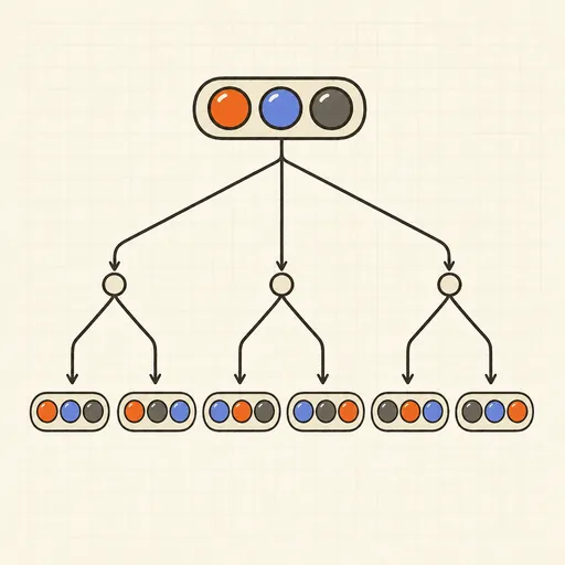
Combinations & Permutations Calculator
nCr and nPr, with and without repetition.
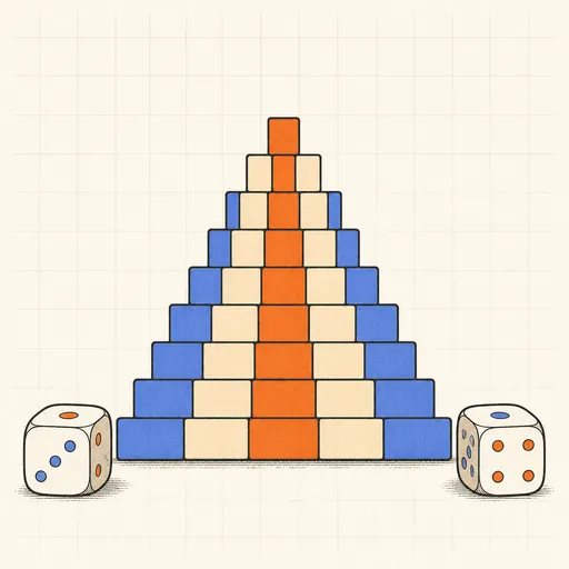
Dice Probability Calculator
Exact sum probabilities for any number of dice.
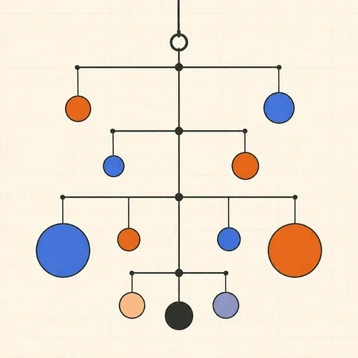
Expected Value Calculator
E[X], variance and SD of a discrete distribution.
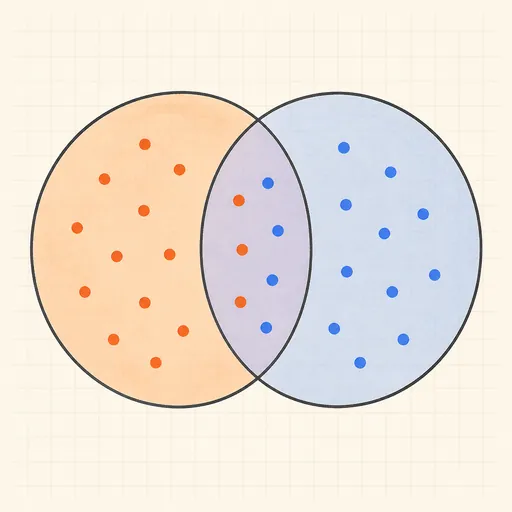
Probability Calculator
Combine independent events, conditional and at-least-once probabilities.

Queueing Theory Calculator (M/M/1, M/M/c)
Waiting times, queue lengths and utilization from arrival and service rates.

Birthday Paradox Calculator
Probability that two people in a group share a birthday.