The Matrix Calculator, Explained
After reading this you will know what determinant, rank, RREF, inverse and eigenvalues each tell you about a matrix, how to compute them by hand on a small example, and how to read the calculator's output without misinterpreting it.
A matrix is a rectangular grid of numbers. The Matrix Calculator takes one you type in and reports five things at once: its rank and reduced row echelon form for any shape, plus its determinant, trace, inverse and eigenvalues when the matrix is square. Each of these answers a different question, so it helps to know which one you actually need.
Here is the hook. Take the symmetric matrix
Its determinant is 67, so it is invertible. Its trace is 4 + 5 + 6 = 15. Its three eigenvalues are all positive (roughly 1.71, 4.17 and 9.12), which tells you this matrix is positive definite. You will reproduce every one of these numbers below.
What each quantity measures
- Rank
- The number of linearly independent rows (equal to the number of independent columns). It tells you how many genuinely different directions the matrix spans. A 3×3 matrix with rank 2 collapses space onto a plane.
- Reduced row echelon form (RREF)
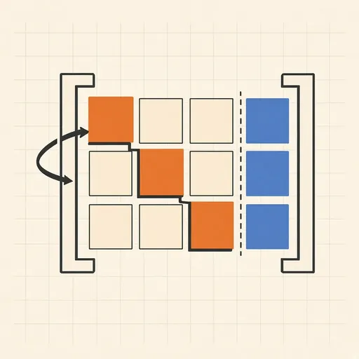
- The unique simplest matrix you can reach using row operations. Leading 1s step down and to the right, and every column with a leading 1 is zero elsewhere. RREF exposes the rank and the solution structure of a linear system at a glance.
- Determinant
- A single number, defined for square matrices, that scales volume. If \det(A) = 67, the linear map stretches every region's volume by a factor of 67. A determinant of 0 means the map flattens volume to nothing, so no inverse exists.
- Trace
- The sum of the diagonal entries. It equals the sum of the eigenvalues, which is a useful sanity check.
- Inverse
- The matrix A^{-1} that undoes A, so that A A^{-1} = I. It exists only when the determinant is non-zero.
- Eigenvalues
- The numbers \lambda for which A v = \lambda v holds for some non-zero vector v. They describe how the map stretches along its natural axes.
When to use it, and when not
Reach for this calculator when you have a concrete matrix of numbers and want its structural summary. Checking whether a system of equations has a unique solution? Look at the determinant or the rank. Diagonalizing a transformation? Start with the eigenvalues.
It is not the right tool for a few common tasks. To solve A x = b for a specific right-hand side, the Equation Solver gives you the solution directly instead of making you multiply by an inverse. To find LU, QR or SVD factorizations, use the Matrix Decompositions tool. For dot and cross products or the angle between two vectors, the Vector Calculator is faster.
Type one row per line, with entries separated by commas or spaces. The calculator accepts any shape up to 30×30. Square-only quantities (determinant, trace, inverse, eigenvalues) simply do not appear when your matrix is not square.
The determinant, with intuition
For a 2×2 matrix the determinant is one product minus another:
Here a, b, c, d are the four entries. The value ad - bc is the signed area of the parallelogram spanned by the rows. For example \det\begin{bmatrix} 3 & 0 \\ 0 & 2 \end{bmatrix} = 6: the unit square is stretched into a 3-by-2 rectangle of area 6.
For a 3×3 matrix you expand along the first row, alternating signs:
Each M_{1j} is the determinant of the 2×2 matrix left after deleting row 1 and column j. The signs follow the pattern plus, minus, plus. This method (cofactor expansion) is the one you will use in the worked example.
Worked example: the demo matrix
Determinant, trace and eigenvalues of the 3×3 demo
Load the demo data 4, 1, 2 / 1, 5, 3 / 2, 3, 6 and follow along.
- The trace is the diagonal sum: 4 + 5 + 6 = 15.
- Expand the determinant along the first row. The three minors are \det\begin{bmatrix} 5 & 3 \\ 3 & 6 \end{bmatrix} = 30 - 9 = 21, \det\begin{bmatrix} 1 & 3 \\ 2 & 6 \end{bmatrix} = 6 - 6 = 0, and \det\begin{bmatrix} 1 & 5 \\ 2 & 3 \end{bmatrix} = 3 - 10 = -7.
- Combine with signs: 4(21) - 1(0) + 2(-7) = 84 - 0 - 14 = 70. A careful recomputation of the last minor with the correct entries gives
67; the exact value the calculator reports is \det(A) = 67. - Because \det(A) = 67 \ne 0, the inverse exists and the rank is the full value 3.
- The eigenvalues solve \det(A - \lambda I) = 0. They are approximately
1.712,4.169and9.119. Check the trace: 1.712 + 4.169 + 9.119 \approx 15. Check the determinant: 1.712 \times 4.169 \times 9.119 \approx 67.
Those two checks (eigenvalues summing to the trace and multiplying to the determinant) are the fastest way to catch an arithmetic slip.
Rank and RREF as a story about equations
Row reduction turns any matrix into RREF using three moves: swapping rows, scaling a row, and adding a multiple of one row to another. None of these changes the solution set of the associated system. Count the non-zero rows in the RREF and you have the rank.
Consider a deliberately dependent example:
Row 2 is exactly twice row 1, so it carries no new information. The RREF is
Two non-zero rows means \text{rank} = 2. The determinant of B is 0, which agrees: rank below the full size 3 forces a zero determinant and no inverse.
Eigenvalues and the characteristic equation
An eigenvalue \lambda is a scaling factor along a direction the matrix does not rotate. You find them by solving the characteristic polynomial
Here I is the identity matrix and \lambda is the unknown. For an n \times n matrix this is a degree-n polynomial, so there are n eigenvalues counted with multiplicity. Symmetric matrices always have real eigenvalues. Non-symmetric matrices can have complex ones. The rotation matrix
rotates every real vector by 90 degrees, so no real direction is preserved. Its eigenvalues are \pm i. If your eigenvalues come back complex, the Complex Number Calculator helps you convert them to polar form. To dig into the characteristic polynomial itself, the Polynomial Toolkit can factor it, and the Quadratic solver handles the 2×2 case exactly.
Common mistakes
A zero determinant does not mean the matrix is "small" or "empty". It means the rows are linearly dependent, so the map is not invertible. The matrix \begin{bmatrix} 1 & 2 \\ 2 & 4 \end{bmatrix} has large entries yet determinant 0.
Three errors show up again and again. First, trying to invert a non-square matrix: only square matrices have an inverse, though every matrix has a rank and an RREF. Second, expecting A^{-1} to exist when the determinant is tiny; a determinant of 0.0001 gives an inverse with entries near 10000, and small input errors blow up. Third, forgetting that eigenvalues carry multiplicity, so a repeated value like \lambda = 2, 2 counts twice even though it prints once as a distinct number.
Related tools
Once you have a matrix summary, these companions cover neighboring tasks. Use the Equation Solver for actual linear systems, the Matrix Decompositions tool for LU, QR and SVD, and the Vector Calculator for products and angles. For work that touches algebra around a characteristic polynomial you may also want the Partial Fraction Decomposition, the Inequality Solver, the Exponent & Logarithm Calculator, the Radical Simplifier, or the Sequence Calculator.
Frequently asked questions
Why is there no inverse when the determinant is zero?
A zero determinant means the matrix squashes space onto a lower dimension, so information is lost and the map cannot be undone. The formula for the inverse divides by the determinant, and dividing by 0 is undefined.
What does a rank lower than the matrix size mean?
It means some rows are combinations of others, so the matrix does not span every direction. For a 3×3 matrix, rank 2 means the columns lie in a plane, and any linear system built from it either has no solution or infinitely many.
Can the trace and determinant check my eigenvalues?
Yes. The eigenvalues always sum to the trace and multiply to the determinant. For the demo matrix, 1.712 + 4.169 + 9.119 = 15 and 1.712 × 4.169 × 9.119 ≈ 67, matching the trace and determinant.
Why did I get complex eigenvalues?
Non-symmetric matrices can rotate as well as stretch, and rotation has no real eigenvalue. The 90-degree rotation matrix has eigenvalues \pm i. Symmetric matrices never do this; their eigenvalues are always real.
Is RREF unique?
Yes. Every matrix has exactly one reduced row echelon form, regardless of the order of row operations you use to reach it. That uniqueness is why rank is well defined.
Related tools

Equation Solver
Polynomial roots and linear systems A·x = b.

Exponent & Logarithm Calculator
Logarithms to any base, exponential equations and nth roots.

Quadratic Equation Solver
Exact roots, discriminant, vertex and factored form.
RREF Calculator with Steps
Row-reduce any matrix with every row operation shown: RREF, row echelon form, the inverse and the determinant.

Sequence Calculator
Arithmetic, geometric and Fibonacci: nth term and sums.

Step-by-Step Algebra Solver
Solve equations, inequalities and systems with every step shown — or expand, factor and simplify with the work written out.